Notes on Band Theory for Sloppy Non-Physicists

May 31, 2020

Motivation

For a non-physicist, the energy band theory for solid materials could get nasty and hard to internalize. But band theory is like a basic languege everybody is fluent with in the community of solit state material research. Therefore, for people like me who is doing research or simply want to learn more advanced physics, we have to grasp the essences of band theory. To my best knowledge there is no textbook of solid-state materials that is designed for pedestrians. Thus, I am making this blog to summarize basic principles that could be of some use for chemists and beginners to research of materials science. This blog is definitely not mathematically vigorous but will performs as a reminder of important stuff about band theory that people could pick it up and read whenever they are lost in the analyses of energy bands. So still basic stuff, no pressure is on.

Band theory: what it is all about?

Once upon a time, there was a guy whose name is Schrodinger and was obssessed with stuff at very small length scale. He came up with an equation named after his name to calculate the energy of basic particles called fermions. The fermion refers to a family of particles among which the most famous one is the electrons. Right after Schrodinger published his out-of-nowhere equation, a group of mathematicians realized that the Schrodinger equation is an eigenvalue problem because it has a general form of:

The solutions \(x\) to such equation are called eigenstates, and each eigenstate corresponds to a specific eigenvalue \(\lambda\). In Schrodinger’s equation \(A\) is usually called “Hamiltonian”. Hamiltonian can takes a form of matrix just like the normal eigenvalue equation, except that the elements in the matrix could be an operator, a function or a constant. The eigenvalues are usually not continuous. They are, as what physicists would like to call it, quantized (a more sexy way to say something is discrete). Let’s again recall the example of electron in an inifinite square potential well, where the electron in the well can only occupy one of discrete energy levels. The energy here is a function of electron’s momentum, and is given by:

where \(k_n=n\pi/L\) is the electron momentum, and \(L\) is the width of potential well. If we plot \(E_n\) against \(k_n\) by varying the \(n\) from -1 to 1, we obtain a energy band made of a set of energy levels in the first Brillouin zone shown below:

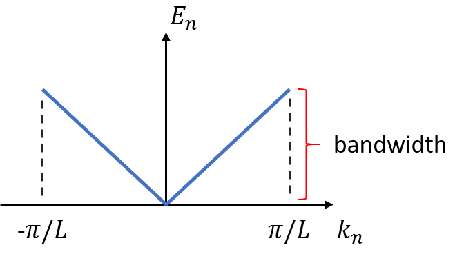
Figure 1. Energy band for electron in infinite square potential well

The difference between the maximum and minimum energy on an energy band is called “bandwidth”. In research of solid state materials or many-body problems, the bandwidth of one energy band or a set of energy bands tells secrets about the properties of solid materials. For instance, in the tight-binding model of 1D lattice, each necleus is strongly bounded by one electron. The energy-momentum relation (dispersion relation) for an electron at nth orbital around a nucleus in such system is given by:

Where \(\epsilon_0\) is a constant and is obtained from the non-perturbative system, and \(a\) is the nucleus spacing distance. With Eq.(2) the band plot now looks different in figure 2:

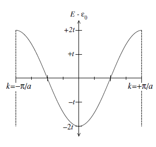
Figure 2. Dispersion of the tight binding 1D chain

Comparing Figure 1 with Figure 2, we see the shape of energy band is changed because of the strong periodic potential environment in the tight-binding model, and also the bandwidth in figure 2 is dependent on the parameter of \(t\). Since \(t\) represents the binding energy between an electron and a nucleus, a narrow bandwidth indicates that a weak binding interaction between electrons and nuclei while the interaction is strong if the bandwidth is wide.

The example above shows that the band structure of electrons changes with external potential environment, and the change in bandwidth implies the changing strength of atomic bonding. From a view of chemistry, the change in band structure can also be interpreted as a result of chemical bond formation. Imagine that at first we have two separate atoms: one has an electron occupying \(1s\) orbital and the other has a \(2p\) electron. The atomic energies at this condition are just \(\epsilon_{1s}\) and \(\epsilon_{2p}\). If we now put the two atoms closer and closer, the atoms start to binding to each other. As a result, the overlap between the \(1s\) orbital and \(2p\) orbital increases, and the probability of electron hopping between the nuclei also increases. Using Eq.(2) we can tell that the increasing orbital overlapping causes the increased value of \(t\). Therefore, the dependence of bandwidth on atomic spacing can be captured in a plot like figure 3.

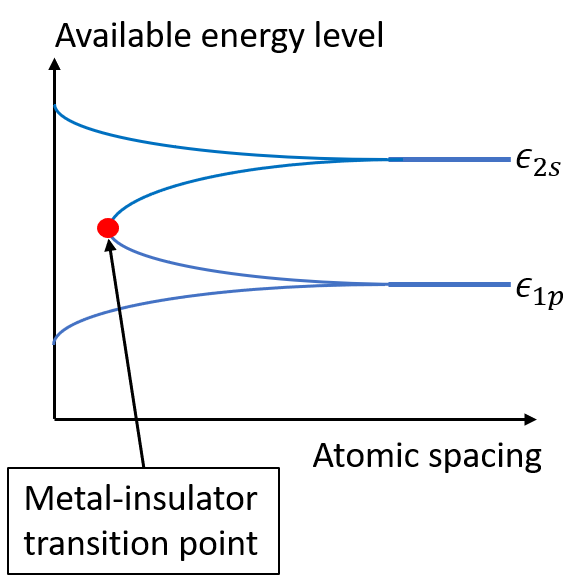
Figure 3. Dependence of bandwidth on interatomic spacing

Metal or Insulator?

As atoms are getting closer in Figure 3, the orbitals emerge and the energies spread to form different bands. Now we can use these energy bands to discuss if a material is a metal or insulator. Going back to our 1D tight-binding system in figure 2, if we have N atoms in the system, the wavefunction of electron can take N different wavelength (i.e. N different values of momentum \(\mathbf{k}\)). Each energy level defined by momentum \(\mathbf{k}\) can only be occupied by two fermions according to Pauli’s exclusion rule. So we have 2N electronic states on the band in figure 2. If each nucleus in our tight-binding lattice chain is monovalent (each atom has one valence electron), the energy band in figure 2 is half-filled. The materials with half-filled bands are metals. If the atoms are divalent, on the other hand, the energy band is fully filled. Since The fulfilled energy band can not carry electron current, the materials with only fulfilled bands are called insulators. The figure 4. shows the half-filled band in figure 2, where the highest energy of filled states is called Fermi energy. The occupied states are stressed in figure 4.

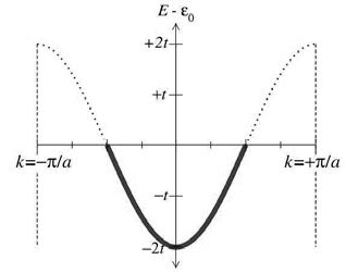
Figure 4. Half-filled energy band

So far we have talked about the differences in band structures of insulator and metal. And we filled our energy band like there is no interaction between the electrons. But that is not true because the Coulombic interaction among electrons could be at level of multiple \(eV\) or even higher. Fortunately, in many cases the ignorance of Coulombic interactions is justified due to the explanation that Lev Landau gave in 1950s. Since it is quite subtle, we are not explaining it here.

Let’s now close this section by talking a little about the semiconductor, or insulator with finite energy band gap. Because the filled energy band does not conduct electronic current, we need electrons to hop from filled bands to empty bands and create holes in the filled bands. Following the convention, we call filled bands in semiconductor as “valence bands” and empty bands as “conducting bands”. The electron hopping in semiconductor is possible through various excitation processes, such as thermal, and optical excitation. Figure 6. shows the electron hopping process between two energy bands of semiconductor:

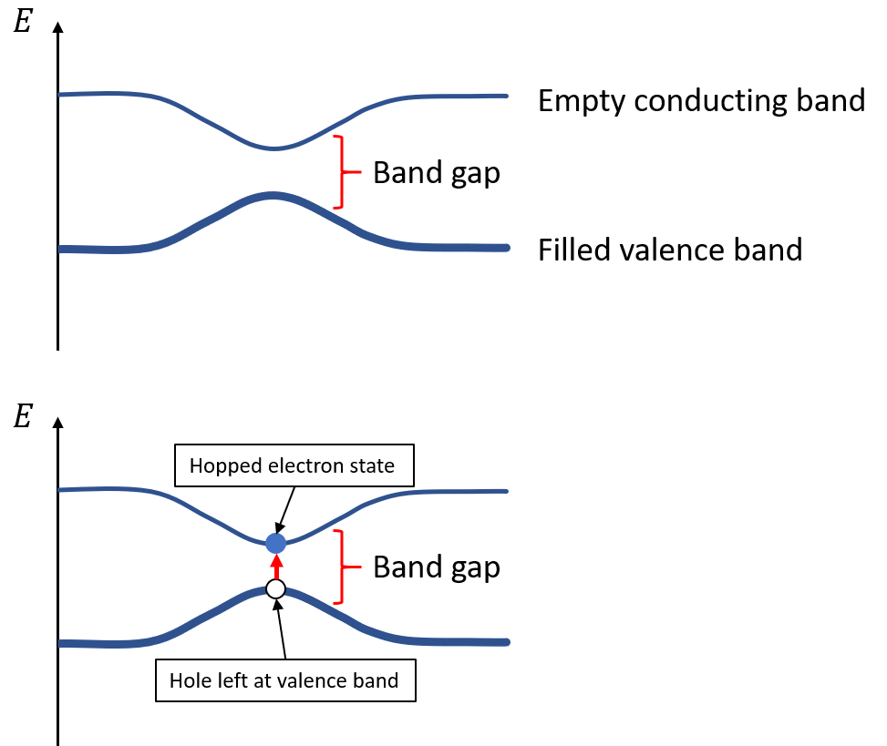
Figure 5. Electron hopping from valence band to conducting band

Fermi surface in first Brillouin zone

Instead of plotting the dispersion relation of occupied states on energy band plot, we can find out the topology of the surface that separates the occupied states and the unoccupied states in first Brillouin zone (FBZ). Such surface is called fermi surface, and all the states(occupied or unoccupied) on the surface are at fermi energy level.

For free electron, the energy is simply \(E=\hbar^2\mathbf{k}/2m\). Setting \(E\) eqaul to fermi energy \(E_f\), it is obvious that the shape of fermi surface is spherical. For metals, the sphere that encloses all the occupied states has a volume that is half of the first Brillouin zone (FBZ), and this spherical space is referred as Fermi sea. When the electron is no longer free and influenced by periodic potential, the fermi surface starts to change its shape based on how strong the external potential is but still encloses half volume of FBZ. How fermi surface changes with the strength of periodic potential is shown in Figure 6. Notice that the filled space is called Fermi sea.

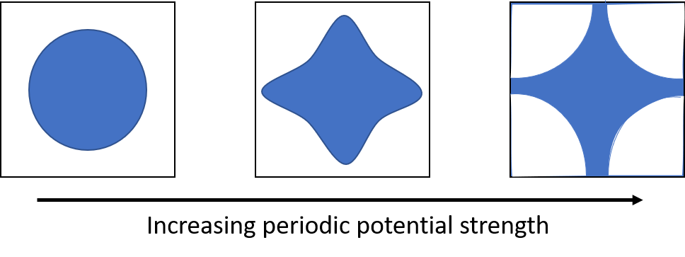
Figure 6. Filled Fermi sea of a square lattice of monovalent atoms in two dimensions as the strength of the periodic potential is varied.

The right subplot in figure 6 shows that the fermi surface is perpendicular to the boundaries of FBZ when it intercepts with the FBZ boundaries. This turns out to be a general rule for both metals and insulators.

When electrons are totally free in insulators, on the other hand, we have a sphere in FBZ that has a volume equal to the volume of FBZ. As the presence of periodic potential becomes stronger, less states outside of FBZ are occupied. Because the reciprocal lattice is periodic, the states that are outside of FBZ correspond to their images in FBZ through “umklapp”.

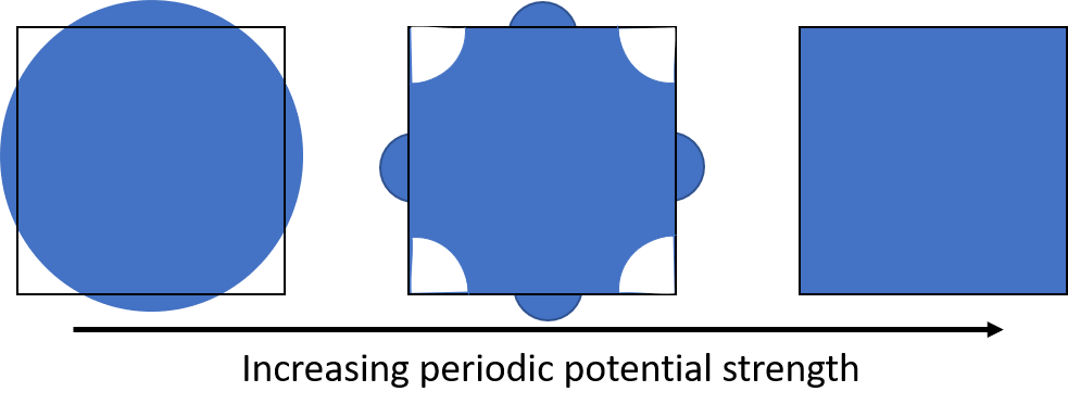
Figure 7. Filled Fermi sea of a square lattice of divalent atoms in two dimensions as the strength of the periodic potential is varied.

A closer look on the middle subplot in figure 7 gives the conclusion that the topology of Fermi surface outside of FBZ distorted comparing to the Fermi surface of free electrons in the left subplot. Using the argument of tight-binding model, we can understand the distortion as the decrease in energies of states due to the binding between electrons and nulei. When a strong periodic potential is added, all of the states are filled and no states outside the first Brillouin zone are filled because of such distortion.

Conclusion

I guess I don’t know how to close this blog yet because there are still a lot I might want to add when the time is right. So keep your eyes on this.