Reciprocal Lattice and Bloch's Theorem

May 17, 2020

Background

I’ve been reading stuff for quite some time, now it’s the time to dive into some real-world problems. One of my current research interests is the many-body effects to conductivity properties of electroactive materials, like the electrode materials used in rechargeable battery and Faradaic desalination cell. More specifically, recent studies proved that the dynamics of polarons, quasi-particles made of a bare electron dressed by its interactions with positive charges and phonons, could be used to explain variation of electronic conductivity in various materials[1]. To study many-body effects in periodic potential environment (i.e., crystal lattice), I will prepare blog articles to refresh and develop a solid understanding of condensed state physics first, then review related concepts/methods from quantum field theory (QFT), and finally hit the details of polaron dynamics. This article is the first step of my possibly long journey to fully understand the polarons.

As an outsider of physics research community, my goal of writing blogs is to make things crystal clear mathematically and physically intuitive. Comments and corrections are equally welcomed.

Bravais Lattice One More Time

First thing is first, Bravais lattice is not crystal lattice. Crystal lattice is atomic base superimposed on one specific kind of Bravais lattice. In other words, Bravais lattice is the bone of crystal lattice while atomic base is the flesh.

For example, the Bravais lattice of NaCl crystal is fcc but the atom base in each primitive cell of fcc lattice contains two atoms: one Na and one Cl.

As a part of material science or physics crriculum, students must’ve learned how to represent points in Bravais lattice, \(\mathbf{R}\), using base vectors \(\mathbf{a}_i\):

The primitive cell of a Bravais lattice is the basic volume that encloses single point of the lattice. We can reproduce the whole lattice by duplicating the primitive cell along the directions of three base vectors without overlapping the cells. When an atomic base is used to describe crystal, the real atoms are occupying the positions that are usually off the point in the Bravais primitive cell. Thus, we need another set of vector, \({\mathbf{r}_i}\), to represent locations of real atoms. Because \(\mathbf{r}_i\) is defined within the primitive cell \(\mathcal{B}\) some people call such vector as “relative coordinates”. Thus, the coordinate of atom “X” in a crystal lattice, \(\mathbf{X}\), is:

From here, the mass distribution of the lattice is given by:

where \(m_i\) is the mass of ith atom. In a perfect crystal lattice where defects and impurity are negligible, the mass distribution is a periodic function, i.e.:

Reciprocal Lattice: Starting from Fourier Expansion

Let \(f(\mathbf{X})\) be a function exhibiting the same periodicity as a Bravais lattice, i.e.

The Fourier expansion of \(f(X)\) is:

Eqn.(3) indicates that

where \(n\in\mathbb{Z}\). To solve for \(\mathbf{k}\) we first define vectors \(\mathbf{b}_i\) that is related to Bravais base vectors \(a_i\) by

If we let

substitute (6) into (4) and use (1),(5) we find

Because \((n_i l_i)\) are definitely integers, we just proved the definition in (6) satisifies (4). The lattice \(\mathbf{Q}\) defined by base vectors \(\mathbf{b}_i\) is the “reciprocal lattice”:

The volume of the Bravais primitive cell is \(V_0=\mathbf{a_1\cdot(a_2\times a_3)}\), from this and (5) we have

Similar things happen to \(\mathbf{b}_2\) and \(\mathbf{b}_3\). One of the most profound properties of reciprocal lattice is that the Fourier component of a periodic function on a Bravais lattice is also periodic on reciprocal lattice except that the periodicity \(\mathbf{R}\) is replaced with reciprocal lattice vecotor \(\mathbf{Q}\). This fact has deep consequences, as we shall see. For instance,we Fourier transform the periodic function \(f(\mathbf{r})\) as:

Now we let \(\mathbf{r}^{\prime}=\mathbf{r+R}\) and give:

where in second step we used \(\mathbf{Q\cdot R}=2\pi n\). Another famous theorem of the complex exponential sum is:

and \(N\) is the number of points in Bravais lattice. We now let \(\mathbf{G}\) as vectors on reciprocal lattice and \(\mathbf{R}\) as vectos on Bravais lattice. From the figure blow, we derive the following relation between the two:

where \(d\) is the distance between the lattice planes in the same plane family shown in the figure.

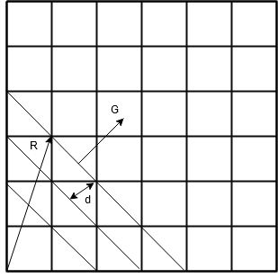
Figure 1. R and G on Bravais Lattice

If we choose \(\|\mathbf{G}\|=\frac{2\pi}{d}\), Eq.(12) is recovered to Eq. (4). Each \(\mathbf{Q}\) in Eq.(7) therefore determines a family of lattice planes with plane interval equal to \(d=\frac{2\pi}{\|\mathbf{Q}\|}\).

First Brillouin Zone

To understand first Brillouin zone, we first introduce the concept of Wigner-Seitz primitive unit cell. Imagine now we select a point,A, in Bravais lattice and its nearest neighbors. We then draw straight lines from A to its nearest neighbors and find the middle points of these lines. In a 3D Bravais lattice let’s further imagine that planes passing through the middle points and perpendicular to the lines enclose a region around point A. This region is called Wigner-Seitz primitive cell. It is not a surprise that the minimum sum of distances from vertices of Bravais primitive unit cell to point A is obtained when the primitive cell is Wigner-Seitz cell. Similarly, the space enclosed by Wigner-Seitz primitive cell on reciprocal lattice is called “First Brillouin zone”. See Fig. 2 for the First Brillouin zone (FBZ) on a 2D reciprocal lattice.

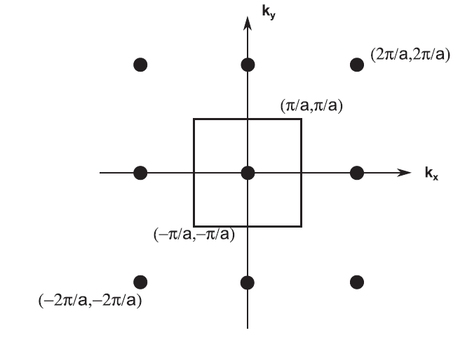
Figure 2. FBZ on a 2D reciprocal lattice

FBZ also plays an important role in understanding X-ray scattering pattern. According to Bragg’s theorem, the wavelength of X-ray is related to the distance between lattice planes by:

The reflection of electromagnetic wave in X-ray scattering process may be described as the incoming photon at state \(\|\mathbf{k}_i\rangle\) interacts with periodic potential \(V(\mathbf{r})\) in crystal lattice and results in the outcoming photon at state \(\|\mathbf{k}_f\rangle\).

For those who have no experience with Dirac notation, \(\|X\rangle\) is used to represent an eigenstate of an Hamiltonian and is called “ket”. Its Hermitian adjoint, \(\langle X\|\) is called “bra”. To give an example of their use, let’s recall the time-independent Schrodinger equation (TISE) as \((-\hbar^2\frac{\nabla^2}{2m}+V(\mathbf{r}))\psi(r)=E\psi(r)\), where \(E\) is the eigenvalue corresponding to the eigenstate \(\psi(r)\). To make TISE more compact, we call \(\mathbf{H}=(-\hbar^2\frac{\nabla^2}{2m}+V(\mathbf{r}))\) as the “Hamiltonian” and now TISE becomes \(\mathbf{H}\|\psi\rangle=E\|\psi\rangle\). Using Dirac notation, the possibility amplitude of transforming state \(\psi_1\) to \(\psi_2\) is simply \(\langle\psi_2\|\mathbf{H\|\psi_1}\rangle\). Note that this amplitude is not a product of eigenstate, Hamiltonian, and another eigenstate, it is a integral. If eigenstates are coordinate-based (\(\psi=\psi(\mathbf{r})\)), \(\langle\psi_2\|\mathbf{H\|\psi_1}\rangle=\int d\mathbf{r}\phi^{\dagger}_2(r)\mathbf{H}\psi_1(r)\), where \({^{\dagger}}\) means Hermitian transpose operation.

Thus, the posibility amplitude of obtaining photon at state \(\|k_f\rangle\) from \(\|k_i\rangle\) through periodic potential field \(V(\mathbf{R})\) is:

as the coordinate-based wavefunctions that satisfy non-relativistic Schrodinger equation has the form of \(e^{i\mathbf{k\cdot r}}\). Because potential function \(V(r)\) is periodic on Bravais lattice, its Fourier transformation (14) must be periodic on reciprocal lattice. Based on the discussion in the previous section, we must have:

which is the “von Laue condition“Let \(\mathcal{BL}\) and \(\mathcal{B}\) represent the point colletions in Bravais lattice and in atom base, respectively. We can write potential function \(V(r)\) as:

substitute (15), (16) into (14), we have:

\(\left\langle\mathbf{k}_{f}|V(\mathbf{r})| \mathbf{k}_{i}\right\rangle=\int d^{3} r e^{-i\mathbf{Q}\cdot \mathbf{r}} \sum_{\mathbf{R} \in \mathcal{B} \mathcal{L}} \sum_{i \in \mathcal{B}} v_{i}\left(\mathbf{r}-\mathbf{R}-\mathbf{r}_{i}\right)\tag{17}\) Let \(\mathbf{r^{\prime}}=\mathbf{r}-\mathbf{R}-\mathbf{r}_{i}\), and (17) becomes

where (10) and (11) are used in the second step of (18). (Don’t be scared by the minus sign in the exponential term, you can treat \(e^{-i\mathbf{QR}}\) as \(e^{i(-\mathbf{Q})\cdot\mathbf{R}}\))

If atom base \(\mathcal{B}\) is constituted by identical atoms, (18) is simply:

where \(S(Q)\) is the famous “geometric form factor”. In an x-ray experiment, the peaks in the reflected beam will occur right at \(\mathbf{k_i +Q}\), with an intensity proportional to \(\|v(\mathbf{Q})\|^2\), with a possible additional modulation by the geometrical form factor.

Bloch’s Theorem

This section is all about Bloch’s theorem, the first symmetry-flavored theorem appears in condensed matter physics textbook, which gives general from of wavefunction for fermions in periodic lattice. We first restate it here and then prove it using three different but related ways in latter subsections.

Bloch’s Theorem: An electron in a periodic potential has eigenstates of the form

An intuitive proof

The proof of Bloch’s theorem given in this section is inspired by Jordan Edmounds’ incredible youtube lecture[2]. Let’s start with a 1D lattice shown below, where atoms are aligned with a interval of \(a\).

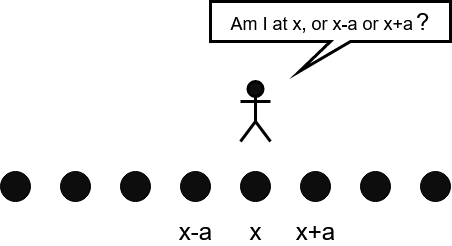
Figure 3. Indistinguishable atom on 1D lattice

Because the identical atoms on a sufficiently long 1D lattice are indistinguishable, the wavefunction of electron \(\Psi(\mathbf{r})\) on such lattice must be periodic:

where \(C\) is the modulation to \(\Psi\). To make sure that \(\|\Psi(\mathbf{r})\|^2=\|\Psi(\mathbf{r+a})\|^2\), we must have \(C^2\equiv1\). We now impose the “periodic boundary condition”(PBC), hence for finite 1D lattice, the PBC indicates the linear lattice becomes a circular lattice shown below:

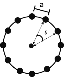
Figure 4. Circular 1D lattice

The use of PBC might sound weird here, but if we think of a real crystal lattice,the dimensions of crystal lattice are infinite comparing to atomic interval. The PBC then indicates an enormous hyperspherical lattice structure and is valid for the parts that are sufficiently far away from the crystal surface.

Using the circular lattice in Fig. 4, we can translate the original wavefunction \(\Psi\) by \(N\) times to go back to the original wavefunction. That is:

Thus, \(C\) must be the Nth root unity. One of the options for \(C\) is \(e^{i2\pi\frac{S}{N}}\), where \(S\in\mathbb{Z}\). Recall that \(\Psi\) is also a function of coordinate on our 1D lattice, so we must have

since

We now define a crystal momentum \(k\) as \(k=\frac{2\pi S}{Na}\), and the wavefunction becomes:

Now the question we have is: is this the only option for \(\Psi\)? Probably not,so we still need to cover the possibility of using other periodic function to construct the wavefunction. To this end, we append a periodic function in (22) and get:

where \(u(r+a)=u(r)\). We use the subscript here to emphasize the use of crystal momentum. (23) can be generalized to high dimension space, and gives:

which is just Bloch’s theorem, Q.E.D.

An Probably important side note: nitice that the crystal momentum of a 1D lattice is defined as \(k=2\pi S/Na\), and the dimension of our hypothetical 1D lattice is \(L=Na\). Thus, the product of \(kr=2\pi Sr/L\) is only important when it is in FBZ. In other words, when \(2\pi Sr/L\) is outside of FBZ, that is \(kr=2\pi n+k^{\prime}r\), we always have a factor of \(e^{i2\pi n}=1\), and the wavefunction essentially corresponds to a crystal momentum \(k^{\prime}\) in FBZ. Similar arguments can be easily applied to high dimensional wavefunction.

Proof using Fourier transformed Schrodinger equation

The proof introduced in this section starts from time-independent Schrodinger equation:

We now write \(V\) and \(\Psi\) in its Fourier expansions:

Substitute (24) in Schrodinger equation, we have

Next, we multiply (25) with \(e^{-ik^{\prime}r}\) and integrate (25) over \(r\) to obtain:

Using the orthogonality of periodic functions, similar to (11):

Cancelling \(V\) we obtain from (26) the Fourier transformation of Schrodinger equation:

In order to solve (28) for eigenvalue \(E\), we have to know all the values of \(c_{k'-G}\). Compare the Fourier expansion with (28), we then conclude that \(\Psi\) can only be related to \(c_{k-G}\) if its Fourier expansion is:

\(\Psi=\sum_{G}c_{k-G}e^{i(k-G)r}=e^{ikr}\sum_Gc_{k-G}e^{-iGr}=e^{ikr}u_k(r)\) Q.E.D.

Proof using translational operators

The proof in this section is prepared for those who know something about quantum-mechanical operators and their embeddied symmetries, more specifically, translation operators and their commutation rules with Hamiltonian. Let’s start with a free electron, whose Hamiltonian is just its kinetic energy:

(29) is obviously invariant under translational transformation as it is not dependent on coordinates. As a consequence, the translational operator

commutes with Hamiltonian. However, when the electron is in a periodic potential \(V(r)=V(r+R)\), such global translational symmetry is broken. But the Hamiltonian now commutes with \(T(\mathbf{R})\). When \(T(R)\) is applied to wavefunction \(\Psi(r)\), we find:

Note that we can let

where \(\mathbf{k}\) is in FBZ. Substitute (32) in (31), we find:

We conclude that, for a periodic potential, all the conserved electron wave-vectors belong to the first Brillouin zone. (33) is sometimes called as “Floquet’s Theorem”. Using Floquet’s theorem, it is followed that

Q.E.D.

Conclusion

Some drunk undergrads are fighting outside when I’m finishing. Please don’t get me wrong, I am indeed hate undergrads and am not willing to teach them any of these things. I write this only to embark a journey that kills my weekend time and fulfills my curiosity.

References

[1] Sio, Weng Hong, et al. “Ab initio theory of polarons: Formalism and applications.” Physical Review B 99.23 (2019): 235139.

[2] https://www.youtube.com/watch?v=8EOReuCrNuE