Qubit Saga: Deutsch–Jozsa Algorithm

September 2, 2023

Tags: [quantum-mechanics] [quantum-algorithms]

北风就从今夜开始，慢慢吹起。

1. Is Your Function Constant?
- 1.1 The Chernoff bound and exponential envelope
2. Quantum Circuit Basics
- 2.1 Single- and multi-qubit gates
- 2.2 Introduction to entanglement
3. Quantum Circuit for Deutsch’s Algorithm
Index

The Deutsch–Jozsa algorithm can be considered as an introductory-level quantum algorithm. Its creation was aimed at demonstrating the superiority of quantum computation in solving a certain class of problems. However, the problem discussed in this article lacks corresponding real-life examples. Therefore, readers might as well regard this algorithm as a deliberate construction by the academic community to prove the quantum supremacy. In this article, starting from the corresponding mathematical problem, the author dissects the quantum circuit behind the Deutsch-Jozsa algorithm.

1. Is Your Function Constant?

The problems efficiently solvable by the algorithm can be described as follows: Given a function $f(x)$, if we do not know its explicit expression, how can we determine whether this function always outputs a constant value? The red line in represents a simple constant function, where $f(x) = 1$ for all values in its domain. The blue line in represents a balanced function, where $f(x) = -1$ when $x < 0$, and $f(x) = 1$ otherwise.

Two function types

In every paper of quantum algorithm, scholars always start with a discussion of how classical computer would solve a problem. Here we take the same route just to fool people that classical algorithms are dumb. We then explain that they are not unbearably bad, just polynomially slower than the quantum algorithm. Without losing the generality, let’s first focus on a function $f(x)$ whose input $x$ is an integer in a range $(-N,N)$, with $N$ being an arbitrary number. Classically, We check if such a function is constant or not by evaluating the function N+1 times. If the evaluated values are all identical, it’s a constant function. Deutsch-Jozsa algorithm tells function type by ensuring a specific quantum state’s probability becomes unity while excluding other possibilities.

1.1 The Chernoff bound and exponential envelope

The classical method above is never used in real life as it’s usually hard to enumerate all possible inputs for discrete or continuous functions. Instead, we want to keep the probability of guessing the wrong function type to a low level, $\epsilon$the $\epsilon$ here should be diminishingly small. . In the case above, we have a function producing non-deterministic binary output $f(x_i)$, and we’re facing a decision problem, i.e., how probable we will guess the function type wrong after $k\ll N/2+1$ function evaluation? Let’s assume, without any loss of generality, that we guess the function type to be constant. With this assumption, the question becomes: what is the possibility of the k evaluations telling me that the function is not constant? In the following discussion, we use $f_i=1$ to represent $f(x_i)=1$ and $f_i=0$ otherwise. After k evaluations by randomly choosing $\{x_0,x_1,...,x_k\}$, the majority voting fails when $s_k=\sum_i^k f_i<k$. we need only one wrong answer to tell the function is not constant There are $C^q_k$ k-sequences $\{f_1,f_2,...,f_k\}$ that have $q$ correct answers, and the probability of $s_k=q$ is

$$\large p(s_k=q)=C^q_k(1/2+\delta)^q(1/2-\delta)^{k-q},$$

in which $p(f_i=1)=\frac{1}{2}+\delta$ and $p(f_i=0)=\frac{1}{2}-\delta$.we introduce $\delta$ here for the sake of generality. Note that for a balanced function $\delta=0$, and $\delta=1/2$ for constant function. Any other function type will have its $\delta\in(0,1/2)$. It is clear that $p(s_k=q)$ follows binomial distribution and the expectation value $E(s_k)=k(1/2+\delta)$. Therefore, the most probable $s_k$ that yields a failed majority voting should be as close to $k(1/2+\delta)$ as possible. However, we don’t know how to choose $\delta$ as the explicit expression of $f(x)$ is unknow to us. An educated guess could be $\delta\cong 0$, that is, assuming that correct or wrong answers are almost equally possible. If we take such an assumption, then each $\{f_1,f_2,...,f_k\}$ with its $s_k=k/2$ can occur with the probability

$$\large p(\{f_1,f_2,...,f_k\}; s_k=k/2+\lim_{\delta\rightarrow0}\delta)=(\frac{1}{2}-\delta)^{k/2}(\frac{1}{2}+\delta)^{k/2}.$$

Since there are $2^k$ possible squences $\{f_1,f_2,...,f_k\}$, we can conclude from that the possibility of guessing function type wrong after $k$ evaluations is

$$\large p(s_k\leq k-1)<2^k(\frac{1}{2}-\delta)^{k/2}(\frac{1}{2}+\delta)^{k/2}=(1-4\delta^2)^{k/2},$$

Note that $1-x\leq \exp(-x)$, we obtain the Chernoff bound:

$$\large p(s_k\leq k-1)<\exp(-2\delta^2k).$$

Let $\epsilon=p(s_k\leq k-1)$, we have the error drops below $\epsilon$ when the number of function evaluations exceeds the following limit:

$$\large k>\frac{1}{2\delta^2}\ln(\frac{1}{\epsilon}).$$

Thus, the problem described here has a classical complexity of $O(\ln(1/\epsilon))$.

There is a another way to calculate the classical complexity using the exponential envolop of $p(s_k\leq k-1)$.this discussion is for people(including me) who are not comfortable with the assumed value of $\delta$ above Because there is only one sequence that has $s_k=k$ with $\{f_1,f_2,...f_k\}=\{1,1,...,1\}$, we have the probability of such a sequence being

$$\large p(s_k=k)=(\frac{1}{2}+\delta)^k$$

and hence,

$$\large p(s_k\leq k-1)=1-p(s_k=k)=1-(\frac{1}{2}+\delta)^k<e^{-k\delta^3}$$

where the last inequality gives an exponential envelope for $p(s_k\leq k-1)$. Repeat the analysis above, we have

$$\large \epsilon<e^{-k\delta^3}\rightarrow k>\frac{1}{\delta^3}\ln(1/\epsilon)$$

giving the same classical complexity as the Chernoff bound. below shows how $p(s_k\leq k-1)$, Chernoff bound, and the exponential envelope in vary with the $\delta$. As we increase the $k$ value, the Chernoff bound breaks at $\lfloor k\rfloor>3$, and the envelope breaks as well when $\lfloor k\rfloor\geq8$. In summary, both bounds hold for the full range of $\delta\in(0,1/2)$ when limited function evaluations are performed.

Interactive plot of $p(s_k\leq k-1)$, Chernoff bound, and exponential envelope varying with $\delta$. Use the slider to see how the $p(s_k\leq k-1)$ goes above the two bounds as k increases.

The analysis in wraps up our problem statement in the context of classical computation. Next we will quickly go through some basics of quantum gates and draft the first quantum circuit for solving the problem here.

2. Quantum Circuit Basics

Transistors give rise to logic circuits by regulating the flow of electric current through varying voltage levels, so the binary states, 1 and 0, are represented physically by voltage levels. Because the voltage is always controllable by logic gates, signals passing through the logic circuit are deterministic. Quantum circuit, on the other hand, is never deterministic as its basic unit is “qubit”, the quantum counterpart of the classical “bit”. Qubits are physical realizations of quantum two-state systems.
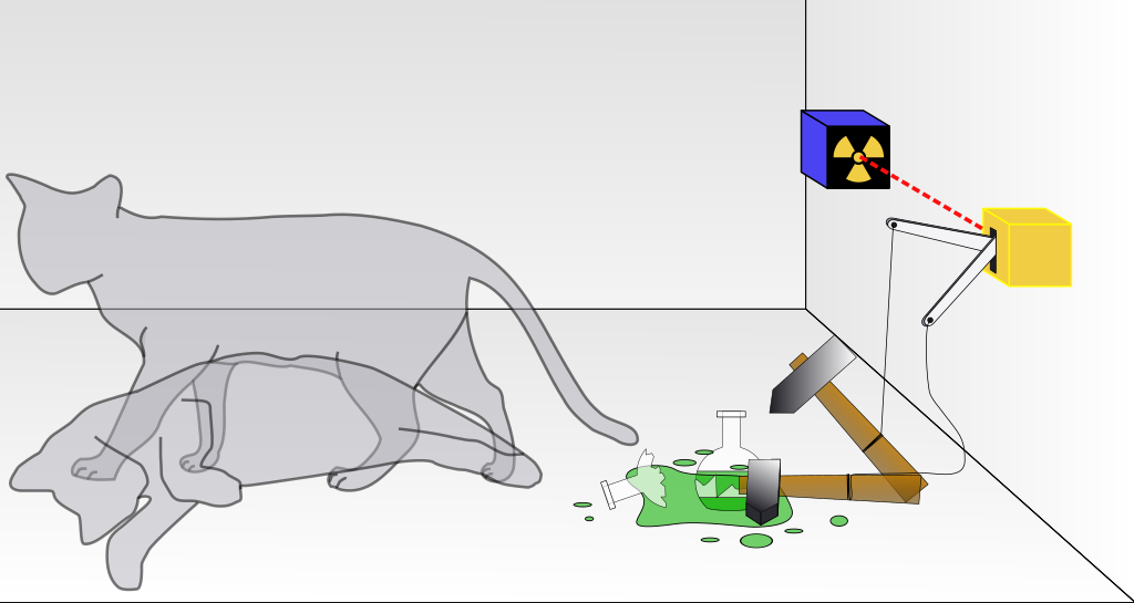
Schrodinger’s cat on Wikipedia For people who are not familiar with quantum mechanics, you can think of qubit as a blackbox containing Schrodinger’s cat. We get to know if the cat is dead or alive by opening the box. Here, dead and alive are the two “quantum states“here we use Dirac notation to represent quantum states. In this case, the cat has two possible states:$\ket{alive}$ or $\ket{dead}$ , and the behavior of opening box is our “measurement” of the cat’s statesfor now, let’s naively use $\hat{M}$ to represent the measurement. In the language of linear algebra, this is an operator applicable to the vector space spanned by basis vectors of $\ket{alive}$ and $\ket{dead}$ . Before the “measurement”, the cat can either be dead or alive. Such a state uncertainty is captured by the concept of superposition. Let’s first use Dirac notation to represent superposition in this case as $\ket{alive}+\ket{dead}$. Notice the ressemblance here between the superposition and the linear combinationIf we treat $\ket{alive}$ and $\ket{dead}$ as two linearly independent vectors, then all of the linear combinations, $\alpha\ket{alive}+\beta\ket{dead}$ forms a vector space. pervasive in linear algebra. At the moment of opening the blackbox, we apply the “measurement” to the superposed state, $\hat{M}(\ket{alive}+\ket{dead})$, which results in $\ket{alive}$ if the cat jumps out of the box, or $\ket{dead}$ if the cat stays there forever. Before the measurement, we can only predict the cat’s state using probabilities. For example, if we place a bottle of poison with the cat in the box, and we know cats like to topple small things. Then the probability of cat being alive at time $t$, $p(\ket{\psi(t)}=\ket{alive})$ should be lower than 1$\ket{\psi(t)}$ represents the cat’s state at time $t$ . Note that $\small p(\ket{\psi(t)}=\ket{alive})+p(\ket{\psi(t)}=\ket{dead})=1$ at any time instance. To reflect this fact in the superposed state, we need to normalize the “length” of the linear combination $\alpha\ket{alive}+\beta\ket{dead}$ to one, i.e., $\alpha^2+\beta^2=1$. For the cat, we have $\small p(\ket{\psi(t)}=\ket{alive})=\lvert\alpha\rvert^2$, and $\small p(\ket{\psi(t)}=\ket{dead})=\lvert\beta\rvert^2$. Due to their relations to probabilities, $\alpha$ and $\beta$ are called probability amplitudes, and they are generally complex numbers.

2.1 Single- and multi-qubit gates

So a qubit can be thought of a blackbox containing a cat of superposed quantum state. Upon the measurement, the qubit has two possible states analogous to the classical bit, $\ket{0}$ and $\ket{1}$. If we first set the qubit at the state of $\ket{0}$ and do nothing(e.g. no poison bottle in the box)Doing nothing is an oversimplified statement. Huge amount of efforts is required to protect a quantum system from noises that break its current state before measurement. , next time when we measure the qubit, it will still be at the state of $\ket{0}$ just like what we would expect on a classical computer. However, we can turn the qubit state into a superposed one by applying quantum gate to itthere are only two effects of classical gates to bits: flip the bit or remain bit state. . Such a gate is call Hadamard gate, and is represented as $\fbox{H}$ in quantum circuit.

The following quantum circuit shows one Hadamard gate applied to one qubit(the horizontal line).

One Hadamard gate,see QC in Quirk. Its probability distribution is shown below

The qubit in is set to $\ket{0}$ at the beginning. The wire represents evolution of the qubit in time, along which we have one intermediate point: m1. The caption of also gives the probabilities of getting different states of q0 at the end. Because the Hadamard gate turns q0 into a superposed state, $1/\sqrt{2}\ket{0}+1/\sqrt{2}\ket{1}$$\alpha=\beta=1/\sqrt{2}$ , we have $(1/\sqrt{2})^2=1/2$ possibility of getting $\ket{0}$ or $\ket{1}$ when measuring the state of q0. The full qubit evolution introduced in can be expressed in Dirac’s notation as

$$\large \hat{H}_{m1}\ket{0}=\frac{1}{\sqrt{2}}(\ket{0}+\ket{1})$$

where subscripts indicate middle points’ locations. If there are multiple gates applied to a qubit, it’s conventional to place operators chronically from right to left before the qubit.

Now, let’s consider two qubits, and add a Hadamard gate to both of them. The corresponding circuit is shown in , and its caption gives 4 possible two-qubit states upon measurement.

Two Hadamard gate,see QC in Quirk. Its probability distribution is shown below

As the symbols indicate, $\ket{00}$ represents the measurement where both q0 and q1 are at $\ket{0}$ while $\ket{01}$ has q0 at $\ket{1}$ and q1 at $\ket{0}$For multi-qubit states, we count indices of individual qubits from right to left. . We can be mathematically rigorous by writting the multi-qubit states using Kronecker products, e.g., $\ket{10}=\ket{1}\otimes\ket{0}$. A more detailed discussion of Kronecker products can be found in my previous post. Kronecker product also enables us to write multi-qubit gates by combining single-qubit gates. For example, the quantum circuit in can be written as

$$\large \hat{H}_{q1}\otimes\hat{H}_{q0}\ket{0}_{q1}\otimes\ket{0}_{q0}=\hat{H}_{q1}\ket{0}_{q1}\otimes\hat{H}_{q0}\ket{0}_{q0}$$

where subscripts are qubits’ indices. Because we always follow the ‘right-first’ convention, can be simplified and expanded as follows:

$$\large \begin{align}\hat{H}\ket{0}\otimes\hat{H}\ket{0}&=\left(\frac{\ket{0}+\ket{1}}{\sqrt{2}}\right)\otimes\left(\frac{\ket{0}+\ket{1}}{\sqrt{2}}\right)\\&=\frac{1}{2}\left(\ket{00}+\ket{01}+\ket{10}+\ket{11}\right)\end{align}$$

The probability amplitudes in are identical for all possible states, and they all correspond to $(1/2)^2=1/4$ possiblity of measured state being one of the four options, agreeing with the result in the caption of .

Another distinct feature of quantum circuits is Controlled gates, which apply quantum gates to a qubit when its control qubit is at state $\ket{1}$. The circuit in shows that $\fbox{H}$ is only applied to q0 when the control qubit q1 has a state of $\ket{1}$.

Controlled Hadamard gate,see QC in Quirk. Its probability distribution is shown below

Nothing happens to q0 as the state of q1 remains at $\ket{0}$ and the $\fbox{H}$ is never triggered. We can use the Pauli-X gate $\fbox{X}$Pauli-X gate is represented by $\bigoplus$ in some circuits. to flip q1 state at m1, and the result is shown in . With q1 state flipped from $\ket{0}$ to $\ket{1}$ at m1, the circuit above applies $\fbox{H}$ to q0, resulting two possible states: $\ket{10}$ and $\ket{11}$.

Controlled Hadamard gate with a Pauli-X gate,see QC in Quirk. Its probability distribution is shown below

We can prove that $p(\ket{01})=p(\ket{11})=0.5$ by progressively following the circuit from left to right.

At m1, we flip q1’s state, $\tiny\hat{X}\otimes\hat{I}\ket{0}\otimes\ket{0}=\hat{X}\ket{0}\otimes\hat{I}\ket{0}=\ket{10}$;
At m2, the Hadamard gate is triggered,

$$\large \small\widehat{CH}\ket{10}=\ket{1}\otimes\left(\frac{\ket{0}+\ket{1}}{\sqrt{2}}\right)=\frac{1}{\sqrt{2}}(\ket{10}+\ket{11}),$$

where $\small\widehat{CH}$ is the controlled Hadamard gate.

Because the probability amplitudes of two possible states in are $\frac{1}{\sqrt{2}}$, the probabilities of getting $\ket{10}$ or $\ket{11}$ are 50% at the end, as the caption of indicates.

2.2 Introduction to entanglement

Now that we have sufficient understanding of single- and multi-qubit operatorswe have used operators and gates interchangeably. , we can move a step furter to see how quantum circuit can create entangled quantum states. Before we give the concept of entanglement, let us take a look at the following circuit:

Making Bell state$$\frac{1}{\sqrt{2}}(\ket{00}+\ket{11})$$, and its probability distribution is shown below

The caption of shows that there are only two possible states: $\ket{00}$ and $\ket{11}$reader can prove this using the progressive method introduced above. with 50% probability for each state. Now, let’s say the measured state of q1 is $\ket{0}$, according to the probability distribution, the two-qubit state must be $\ket{00}$ and q2 must be $\ket{0}$ as well. On the other hand, if q1 is $\ket{1}$, we must have q2 being $\ket{1}$. Thus, states of the two qubits are coupled, and we can confirm the states of both qubits by measuring only one of them. Such a correlation is called quantum entanglement. As a matter of fact, the entangled state $\frac{1}{\sqrt{2}}(\ket{00}+\ket{11})$ is one of the four Bell states. is an interactive circuit to which you can add and delete gates. You can apply $\fbox{X}$ at m1 to q1 to get another Bell state: $\small\frac{1}{\sqrt{2}}(\ket{00}-\ket{11})$, resulting the same probability distribution. On the other hand, if $\fbox{X}$ is applied at m2 to q2, you get $\small\frac{1}{\sqrt{2}}(\ket{01}+\ket{10})$. If two $\fbox{X}$ are applied at m1 to q2 and q1, we get the last Bell state $\small\frac{1}{\sqrt{2}}(\ket{01}-\ket{10})$.

Bell states introduced here belong to a class of entangled qubit states, called maximally entangled states. The name is due to the 100% certainty of one qubit’s state if we know the state of the other one. There are states partially entangled. As an example, consider the state of $\frac{1}{10}\ket{01}+\frac{\sqrt{99}}{10}\ket{00}$. Kronecker product allows us to factor the state into a form of $\ket{0}(\frac{1}{10}\ket{1}+\frac{\sqrt{99}}{10}\ket{0})$. The measurement of q2 will always gives $\ket{0}$, but we have 1% chance of getting $\ket{1}$ and 99% chance of getting $\ket{0}$ for q1. We can NOT tell, with 100% certainty what state q1 is upon the measurement of q2.

3. Quantum Circuit for Deutsch’s Algorithm

Our problem is to find out if a given function is constant or not without knowing its expression. In reality, this could happen if the function is too complicated to figure out its output pattern. For the sake of demonstration, however, we need to construct a simple function in our quantum circuit which maps various inputs to either the same output or different outputs. By constructing the function, we definitely know if it’s constant or not. But imagine you inherit a function constructed previously that takes tens or even hundreds of inputslet’s hope this happens in the near future. , and you can still use Deutsch-Jozsa algorithm to decide function type without sacrificing computational efficiency.

3.1 Construct a function in quantum circuit

A function is a map from a set of inputs to a set of outputs. On a quantum circuit that envolves multiple qubits, a function is a segment between two intermediate points that transform one set of multi-qubit states into another set. In quantum circuit, we use two DIFFERENT sets of qubits as inputs and outputs. For example, If we treat q0 and q1 as input qubits and q2 as output qubit in , then the circuit represents a constant function that always gives $\ket{1}$ at q2 no matter how you prepare inputs at q0 and q1.

A constant function $$f_c(x)$$ that takes inputs at q0 and q1 and output at q2,see QC in Quirk. Its probability distribution is shown below

We can use controlled gates to construct a balanced function as shown in . The function is indeed balanced as $\ket{00}$ and $\ket{11}$ results in $\ket{1}$ at q2 while $\ket{01}$ and $\ket{10}$ maps to $\ket{0}$.

A balanced function $$f_b(x)$$ that takes inputs at q0 and q1 and output at q2,see QC in Quirk. Its probability distribution is shown below

For circuits that implement complicated functions, it is a common practice to hide function details by wrapping corresponding circuit segments into a composite gate. Multi-qubit gates wrapped in this way are called oracle. For the 2-qubit constant function above, an oracle is created in , i.e., the blue block, which always results in $\ket{1}$ at q2, and takes q0 and q1 as function arguments.

An oracle that hides details of the constant function,see QC in Quirk. Its probability distribution is shown below

In the next section, we will use constant and blanced functions introduced here to demostrate Deutsch-Jozsa algorithm, which can tell the two functions apart with 100% confidence.

3.2 Build the circuit before the Hadamard transform

The circuits in shows how Deutsch-Jozsa algorithm is applied to the constant $f_c(x)$. To apply the algorithm to a function of arbitrary number of arguments, you need to replace the oracle in the circuits below with the function and apply the Hadamard gates to all its input qubits before the oracle and apply to them again the Hadamard gates after the oracle.

The Deutsch-Jozsa Algorithm for checking the type of $$f_c(x)$$. The information measured at q1 and q2 is stored at two classical bits, c0 and c1,see QC in Quirk. Its probability distribution is shown below

Let us go back to the basics to analyze what the circuit does. First of all, we have three qubits that serve two different purposes:

function arguments are provided by q0 and q1,
function output is given at q2 but it is initialized with a state of $\frac{\ket{0}-\ket{1}}{\sqrt{2}}$, the qubit q2 is also called ancilla in literatureancilla qubits are used for storing partial results or creating entanglement. .

We can again use the progressive method in Sec.2.1 to see how the multi-qubit state evolves at each intermediate point in . With $\fbox{H}$ at q0 and q1, and $\fbox{X}$ at q2, we turn $\ket{000}$ into the following state at m1:

$$\large \begin{align} \ket{\psi}_{m1}&=\frac{(\ket{0}+\ket{1})}{\sqrt{2}}\otimes\frac{(\ket{0}+\ket{1})}{\sqrt{2}}\otimes\ket{1}\\\\ &=\frac{1}{2}(\ket{00}+\ket{01}+\ket{10}+\ket{11})\otimes\ket{1} \end{align},$$

where the Kronecker products bridge the states at input and output qubits. The second line in indicates that the input qubits are turned into superposed states, including all the possible inputs. This manifests the power of quantum computing, that is, evaluating all possible outputs of a function by feeding it a superposed state composed of all possible inputs. To make our discussion concise, let us write the superposed state as

$$\large \begin{align} \ket{\psi}_{m1}&=\sum_{x=0}^{2^n-1}\frac{1}{\sqrt{2^n}}\ket{x}\otimes\ket{1} \end{align},$$

where we convert the 2-digit binary number(00,01,10,11) into decimal numbers $x$, and $n$ is the number of input qubits in . The conversion simplifies the notation of quantum state evaluated at m2, where we apply $\fbox{H}$ to q3 to give

$$\large \ket{\psi}_{m2}=\sum_{x=0}^{2^n-1}\frac{1}{\sqrt{2^n}}\ket{x}\otimes\frac{\ket{0}-\ket{1}}{\sqrt{2}}.$$

The critical step happens at m3 where we apply the oracle to the three qubits, which results in a state of $\small \ket{f(x)\oplus0}-\ket{f(x)\oplus1}/\sqrt{2}$ at q2. The $\oplus$ within $\ket{ }$ here is the add modulo 2, so $\small\ket{f(x)\oplus0}-\ket{f(x)\oplus1}=(-1)^{f(x)}(\ket{0}-\ket{1})$. With this reasoning, the state at m3 becomes

$$\large \begin{align}\ket{\psi}_{m3} &=\sum_{x=0}^{2^n-1}\frac{1}{\sqrt{2^n}}\ket{x}\otimes\frac{\ket{f(x)\oplus0}-\ket{f(x)\oplus1}}{\sqrt{2}} \\ &=\sum_{x=0}^{2^n-1}\frac{1}{\sqrt{2^n}}\ket{x}\otimes(-1)^{f(x)}\frac{\ket{0}-\ket{1}}{\sqrt{2}}\\ &=\sum_{x=0}^{2^n-1}(-1)^{f(x)}\frac{1}{\sqrt{2^n}}\ket{x}\otimes\frac{\ket{0}-\ket{1}}{\sqrt{2}} \end{align}$$

Thus, the oracle at m3 adds a global phase $(-1)^{f(x)}$ to $\ket{\psi}_{m3}$global phase is a complex number of unity norm attached to a quantum state, and it does not affect probability distribution of the state measurements. . Due to the commutativity between Kronecker product and scalar product, we can move the global phase in front of any qubit(e.g. the last line in ), and such a manipulation is also referred as phase kickback. Because of this, An oracle with its output qubit initialized with the superposed state of $\frac{\ket{0}-\ket{1}}{\sqrt{2}}$ is also referred to as phase oracle.

At this point, we can confidently disregard q2 in the discussion below as its state will remain the same after m3, and $\ket{\psi}_{m3}$ is simplified into

$$\large \ket{\psi}_{m3}=\sum_{x=0}^{2^n-1}(-1)^{f(x)}\frac{1}{\sqrt{2^n}}\ket{x}$$

The step at m4 reveals the function type by applying Hadamard gates(i.e. $\hat{H}\otimes\hat{H}=\hat{H}^{\otimes n}, n=2$) again to the input qubits. Before we derive the final result, we need to take a deeper look at what $\hat{H}^{\otimes n}$ could do to states like $\ket{\psi}_{m3}$.

3.3 Hadamard transform at the last step

Let $k$ be a n-length binary string and $\ket{k}$ be a n-qubit state, then the Hadamard transform gives

$$\large \hat{H}^{\otimes n}|k\rangle=\frac{1}{\sqrt{2^n}} \sum_{j=0}^{2^n-1}(-1)^{k \cdot j}|j\rangle,$$

where $j \cdot k=j_0 k_0 \oplus j_1 k_1 \oplus \cdots \oplus j_{n-1} k_{n-1}$ is the sum of the bitwise product, where $\oplus$ is addition modulo 2. We will try to derive from the perspective of basis transformation, inspired by the blog hereyou need knowledge of group theory in order to fully appreciate the writing . We begin our derivation by considering the simple case of $\small\ket{k}=\ket{\underbrace{00...0}_{n}}$, i.e.,

$$\large \begin{align} \hat{H}^{\otimes n}|\underbrace{00...0}_{n}\rangle&=\frac{1}{\sqrt{2^n}}\prod^{n}(\ket{0}+\ket{1})\\ &=\frac{1}{\sqrt{2^n}}\sum_{z=0}^{2^n-1}\ket{z} \end{align}$$

Now, let’s take a step further by replacing the j-th 0 of $\ket{k}$ with 1, and the Hadamard transform of this modified state is then

$$\large \begin{align} \small \hat{H}^{\otimes n}|\underbrace{00...0}_{n-j}\rangle\otimes\ket{1\underbrace{00...0}_{j-1}}&=\small \frac{1}{\sqrt{2^n}}\prod^{n-j}(\ket{0}+\ket{1})\times (\ket{0}-\ket{1})\times \prod^{j-1}(\ket{0}+\ket{1})\\ &=\small \frac{1}{\sqrt{2^n}}\sum_{z_j=0}\ket{z}-\frac{1}{\sqrt{2^n}}\sum_{z_j=1}\ket{z}\\ &=\small \frac{1}{\sqrt{2^n}}\sum_{z=0}^{2^n-1}(-1)^{k_j\cdot z_j}\ket{z}. \end{align}$$

Since $k_j=1$ in this case, $(-1)^{k_j\cdot z_j}=1$ in when $z_j=1$. When both j-th and l-th 0 of $\ket{k}$ become 1, one can follow the same procedure in to find that

$$\large \begin{align} \small\hat{H}^{\otimes n}\ket{\underbrace{00...0}_{n-l}}\otimes\ket{1\underbrace{00...0}_{l-j-1}}\otimes\ket{1\underbrace{00...0}_{j-1}}&=\small \frac{1}{\sqrt{2^n}}\sum_{z=0}^{2^n-1}(-1)^{k_j\cdot z_j+k_l\cdot z_l}\ket{z}\\\\ &=\small \frac{1}{\sqrt{2^n}}\sum_{z=0}^{2^n-1}(-1)^{k\cdot z}\ket{z}, \end{align}$$

where the last equivelance is due to the fact of digits being 0 in $\ket{k}$ other than $k_j$ and $k_l$. So we must have $k_j\cdot z_j+k_l\cdot z_l=\sum_ik_i\cdot z_i=k\cdot z$, with $k\cdot z$ being the inner product of two binary sequences. The formalism of can also apply to n-length binary sequence $\ket{k}$ with arbitrary number of 1. Also, what matters here is only the oddity of $\sum_ik_i\cdot z_i$, we can modify the inner product by using the addition modulo 2, that is, $k\cdot z=k_0z_0\oplus k_0z_0\oplus\cdots k_nz_n$. With this modification, we now complete the derivation of Hadamard transform in .

Applying to gives

$$\large \begin{align} \hat{H}^{\otimes n}\ket{\psi}_{m3}&=\sum_{x=0}^{2^n-1}(-1)^{f(x)}\frac{1}{\sqrt{2^{2n}}}\sum_{z=0}^{2^n-1}(-1)^{x\cdot z}\ket{z}\\ &=\sum_{z=0}^{2^n-1}\sum_{x=0}^{2^n-1}(-1)^{f(x)+x\cdot z}\frac{1}{2^{n}}\ket{z}. \end{align}$$

Note that $\ket{z}$ represents possible state of input qubits, and each possible state has its probability amplitude being $\small \sum_{x=0}^{2^n-1}(-1)^{f(x)+x\cdot z}\frac{1}{2^{n}}$. For a constant function that $f(x)\equiv1$, we have the probability of $\small\ket{z}=\ket{\underbrace{00..0}_{n}}$ being unity because $f(x)+x\cdot z\equiv 1$ for all the $2^n$ terms. On the other hand, $\small \sum_{x=0}^{2^n-1}(-1)^{f(x)+x\cdot z}\frac{1}{2^{n}}\equiv0$ if $f(x)$ is balanced.

To verify the statement above, we can replace $f_c(x)$ in with $f_b(x)$ as shown in

Erroneous implementation of the Deutsch-Jozsa Algorithm for checking the type of $$f_b(x)$$,see QC in Quirk. Its probability distribution is shown below

Indeed, the balanced function guarantees the input qubits at a state of $\ket{11}$ at the end. With the Deutsch-Jozsa algorithm, we can tell for sure that the function is not constant if at least one measured state is not $\ket{\underbrace{00...0}_{n}}$.

3.4 Running into mistake with extra ancilla

The circuit in is my first implementation of the algorithm, in which 4 quibits, instead of 3 qubits, were employed. I was doing so to enforce “$\ket{y\oplus f(x)}$” at q3, as indicated by public references.

Erroneous implementation of the Deutsch-Jozsa Algorithm for checking the type of $$f_b(x)$$,see QC in Quirk. Its probability distribution is shown below

The newly added q3 results in the following $\ket{\psi}_{m2}$ that has an extra $\ket{f(x)}$ compared to ,

$$\large \ket{\psi}_{m2}=\sum_{x=0}^{2^n-1}\frac{1}{\sqrt{2^n}}\ket{x}\otimes\ket{f(x)}\otimes\frac{\ket{0}-\ket{1}}{\sqrt{2}}.$$

By following the steps in , the quantum state at m3 becomes

$$\large \ket{\psi}_{m3}=\sum_{x=0}^{2^n-1}(-1)^{f(x)}\frac{1}{\sqrt{2^n}}\ket{x}\otimes\ket{f(x)}.$$

After the Hadamard transform, we can no longer guaranttee zero probability of getting $\ket{\underbrace{00...0}_{n}}$ for the balanced function as

$$\large \begin{align} \ket{\psi}_{m4}&=\sum_{x=0}^{2^n-1}(-1)^{f(x)}\frac{1}{\sqrt{2^{2n}}}\sum_{z=0}^{2^n-1}(-1)^{x\cdot z}\ket{z}\otimes\ket{f(x)}\\ &=\sum_{z=0}^{2^n-1}\sum_{x=0}^{2^n-1}(-1)^{f(x)+x\cdot z}\frac{1}{2^{n}}\ket{z}\otimes\ket{f(x)}. \end{align}$$

Therefore, states like $\ket{0000}$ and $\ket{0100}$ have their probabilities being 12.5%, as indicated in the caption of .