Fermi and Coulomb Holes
August 28, 2020
The “hole” in density functional theory (DFT) refers to the depletion of electron density around a reference spatial point, as a result of exchange-correlation effects among electrons. To see how the holes emerge in the formulation of DFT, let us start with the definition of charge/electron density:
\[\rho(\vec{x_1})=N \int d \vec{x_2} \dots d \vec{x_N}|\psi(\vec{x_1} \dots \vec{x_N})|^{2}\tag{1}\]where \(N\) and \(\psi\) are the number of electrons and the N-particle wavefunction, and the coordinate of each electron \(\vec{x_i}\) includes spatial and spin information, i.e. \(\vec{x_i}=\{r_i,\sigma_i\}\). The charge density around \(\vec{x_1}\) is essentially the possibility of finding an electron at \(\vec{x_1}\). Thus, the prefactor \(N\) comes from the distinguishability of N electrons in the system.
We can further define a pair probability of finding two electrons at \(\vec{x_1}\) and \(\vec{x_2}\) simultaneously as
\[\rho\left(\vec{x}_{1}, \vec{x_2}\right)=N(N-1) \int d \vec{x_3} \cdots d \vec{x_N}|\psi|^{2}\tag{2}.\]Using (1) and (2) the conditional probability of finding an electron at \(\vec{x_2}\) when a reference electron is at \(\vec{x_1}\) is then
\[\Omega\left(\vec{x}_{2} ; \vec{x}_{1}\right)=\frac{\rho\left(\vec{x_2}, \vec{x_1}\right)}{\rho\left(\vec{x}_{1}\right)}\tag{3}.\]It is easy to see that
\[\int \Omega\left(\vec{x}_{2} ; \vec{x_1}\right) d \vec{x}_{2}=N-1\tag{4}.\]If electrons in a system are uncorrelated, applying the independence principle of statistics gives
\[\rho(\vec{x_2},\vec{x_1})=\rho(\vec{x_1})\rho(\vec{x_2}),\]but the existence of exchange correlation among the electrons indicates that
\[\rho\left(\vec{x_1}, \vec{x_2}\right)=\rho\left(\vec{x}_{1}\right) \rho\left(\vec{x_2}\right)\left[1+f\left(\vec{x_1} ; \vec{x}_{2}\right)\right]\tag{5}\]where \(f(\vec{x_1};\vec{x_2})\) is the so-called “correlation term” which leads to the depletion of electron density at reference point of \(\vec{x_1}\). The correlation term is usually defined through “exchange-correlation hole”, \(h_{xc}\), i.e. the density difference between the \(\Omega(\vec{x_1};\vec{x_2})\) and \(\rho(\vec{x_2})\):
\[h_{xc}\left(\vec{x_1} ; \vec{x_2}\right)=\frac{\rho\left(\vec{x_2}, \vec{x_1}\right)}{\rho(\vec{x_1})}-\rho\left(\vec{x}_{2}\right)=\rho(\vec{x_2})f(\vec{x_1};\vec{x_2})\tag{6}.\]Because the electronic correlation causes the depletion of the electron density, we have
\[h_{xc}(\vec{x_1};\vec{x_2})<0\tag{7}\]and
\[\int h_{x c}\left(\vec{x_1} ; \vec{x_2}\right) d \vec{x}_{2}=-1\tag{8}.\]The “exchange-correlation” hole is also referred as the total hole because it cancels the self-interaction of the electrons as a result of electron-electron coulombic interactions in the many-body Hamiltonian. The Coulombic interaction among the electrons is given by the following expectation,
\[\left\langle\psi\left|\frac{1}{2} \sum_{i\neq j}^{N} \frac{1}{r_{ij}}\right| \psi\right\rangle=\frac{1}{2} \iint d \vec{r_1} d \vec{r_2} \frac{\rho\left(\vec{r_1},\vec{r_2}\right)}{r_{12}}\tag{9}\]where the spin degree of freedom is already integrated. Using Eq.(6) in (9) we have
\[\left\langle\psi\left|\frac{1}{2} \sum_{i\neq j}^{N} \frac{1}{r_{ij}}\right| \psi\right\rangle=J[\rho]+\frac{1}{2}\iint d\vec{r_1}d\vec{r_2}\frac{h_{xc}\left(\vec{r_1}, \vec{r_2}\right) \rho\left(\vec{r}_{1}\right)}{r_{12}}\tag{10},\]where
\[J[\rho]=\frac{1}{2} \iint \frac{\rho(\vec{r_1}) \rho(\vec{r_2})}{r_{12}} d \vec{r_1} d \vec{r_2}\tag{11}.\]It is easy to see that \(J[\rho]\) contains the self-interaction energy because \(J[\rho]\neq0\) even there is only one electron in the system. Therefore the second term in (10) cancels the self-interaction and accounts for exchange correlation effects. In most DFT calculation packages \(h_{xc}\) is divided into two parts, Fermi hole and Coulomb hole,
\[h_{xc}(r_1;r_2)=h_x^{\sigma_1=\sigma_2}(r_1;r_2)+h_c^{\sigma_1\neq\sigma_2}(r_1;r_2)\tag{12}.\]The Fermi hole echoes Pauli’s exclusion principle wherein two electrons with the same spin state are not allowed to occupy the same spatial location. Therefore the Fermi hole depletes exact one electron near a reference point \(r_1\), i.e.,
\[\int h_{x}\left(\vec{r}_{1} ; \vec{r_2}\right) d \vec{r_2}=-1\tag{13}\]and
\[h_{x}\left(\vec{r_2}\rightarrow\vec{r_1} ; \vec{r_1}\right)=-\rho\left(\vec{r}_{1}\right)\tag{14}.\]Eq.(13) and (14) depict the general shape of Fermi hole in a fermion system. For any electron at \(\vec{r_1}\) Eq.(14) indicates that the distribution of Fermi hole concentrates near the reference point. As \(\|r_1-r_2\|\gg1\) the existence of Fermi hole becomes negligible. Because of this, the charge density distribution under the influence of Fermi hole alone is overly diffusing and the attraction between the electron and the nucleus is screened. Take the hydrogen molecule as a example, when the distance between the two nuclei \(d_{HH}\rightarrow\infty\), the two electrons have the same spin state and the Fermi hole depletes half of the electron density near each neucleus.
Comparing (13) with (8) gives
\[\int h_{c}\left(\vec{r}_{1} ; \vec{r}_{2}\right) d \vec{r}_{2}=0\tag{15}.\]The identity of (15) should not be a surprise as
\[\begin{aligned}\rho^{\sigma_1\neq\sigma_2}(\vec{x_1};\vec{x_2})&=\rho(\vec{x_1})[\rho(\vec{x_2})+h_c(\vec{x_1};\vec{x_2})]\\ \int d\vec{x_2}\rho^{\sigma_1\neq\sigma_2}(\vec{x_1};\vec{x_2})&=N_{\sigma_2}\rho(\vec{x_1}) \end{aligned}\]where Eq.(6) and (12) are used. The \(N_{\sigma_2}\) in the second equation above implies that the probability of finding an electron at \(\vec{r_1}\) with \(\sigma_1\) has nothing to do with finding another electron with \(\sigma_2\neq\sigma_1\) anywhere in the system.
Eq.(15) also indicates that there are some regions in arbitrary many-fermion system where \(h_c>0\). Because the coulombic hole derives from the coulombic interaction, \(h_c\), like \(h_x\), depletes the charge density near a reference charge. Due to the singularity of the Coulombic potential \(r_{12}^{-1}\) at \(r_1=r_2\), the \(h_c(r_1;r_1)\) must satisfy the Kato cusp condition. Therefore, \(h_c>0\) when \(\|r_1-r_2\|\gg0\).
To visualize the above discussion we show in Figure below the Fermi, Coulomb and total exchange-correlation holes for \(H_2\) at various distances. The probe electron is placed at 0.3 bohr to the left of the right proton. We see immediately – in particular for large r – that while both components of the hole are delocalized, the sum of the two, i. e., the total hole, is localized at the proton of the reference electron.hole. The result is a total hole that removes exactly one electron from the right proton as it should in order to yield two undisturbed hydrogen atoms in the dissociation limit.
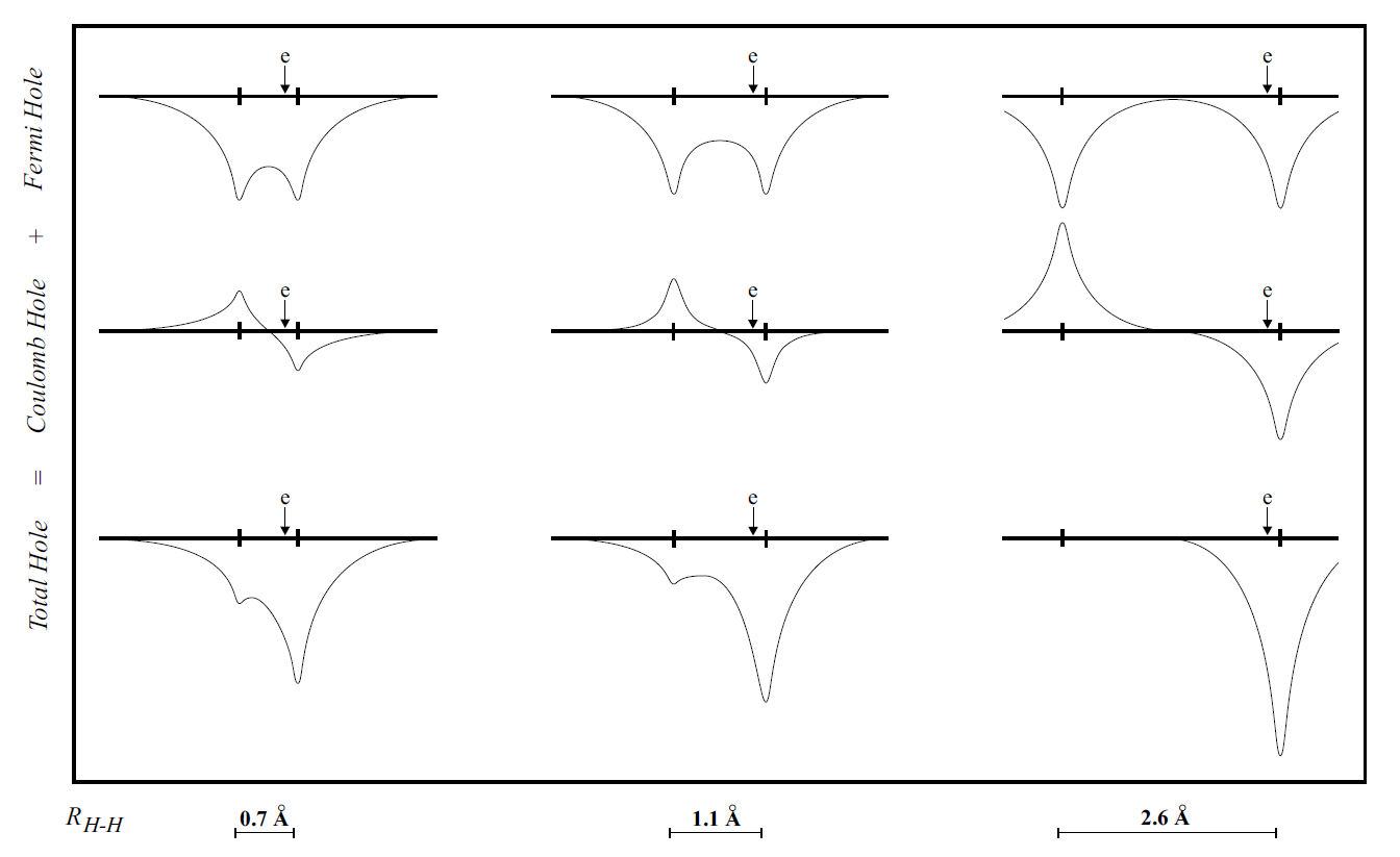
Figure. Fermi, Coulomb and the resulting total exchange-correlation holes for H2 at three different internuclear distances; the position of the probe electron is marked with an arrow (adapted from Baerends and Gritsenko, J. Phys. Chem. A, 101, 5390 (1997))