Landau and Frohlich, The Beginning of the Polaron

June 15, 2020

Background

The polaron theory will be an important part of my final thesis work. I’m writing this to make sure I own every piece of my research proposal that I need to submit to my prelim committee. The blog is divided into three parts. In the first part I will explain the idea of polaron using Landau’s very first phenomenological theory. The second part develops a simple model to calculate the effective mass and size of the polaron. The results from Landau’s theory will be further developed in the last part to derive a quantized Hamiltonian (i.e. Frohlich’s Hamiltonian).

Landau’s Polaron

The idea of polaron is that a free electron, attacted by a positively chaged particle, creates a positively charged “hole” around it through Coulombic interactions with nuclei. As a reseult, the electron is self-trapped by the potential well induced by itself. The effect of polaron may be quanlitatively described by comparing the field energy of adding a free electron in a dielectric continuum with that in vacuo where the dielectric constant \(\varepsilon=1\). Based on this argument, we will derive an expression for the binding energy of an electron to a dielectric medium.

Brief review of electric displacement field

When a dielectric material is placed in an electric field with strength equal to \(\mathbf{E}\), the charge distribution around each atom in the material would become polarized (see Fig 1) and the atoms are no longer neutral.

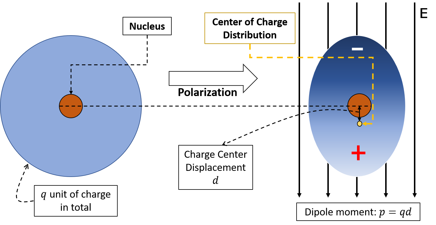
Figure 1. Charge Polarization in Dielectric Continuum

The extent to which the molecules or atoms in dielectric continuum are polarized is described by the dipole moment \(\mathbf{p}\): the product of charge center displacement \(\mathbf{d}\) and total amount of charge \(q\), i.e. \(\mathbf{p}=q\mathbf{d}\). If there are \(N\) molecules or atoms in each unit cell of the dielectric, then the electric polarization (the dipole moment per unit volume) \(\mathbf{P}\) is give by:

One of the interesting things about \(\mathbf{P}\) is its divergence \(\mathbf{\nabla\cdot P}\), as we shall now discuss. Imagine we have a dielectric continuum in which the number density of atoms \(n\) varies with spatial coordinates, i.e. \(n(x,y,z)\), and each nucleus is balanced by \(q\) unit of electron charges. If we considers an infitestimal cube in the dielectric with spatial coordinates in a range from \((x,y,z)\) to \((x+dx,y+dy,z+dz)\), then the total amount of electron charge in such cube is:

When we apply an electric field \(\mathbf{E}\) on the dielectric, the electron charge centers shift off their original positions by a vector \(\mathbf{\vec{d}}=(d_x,d_y,d_z)\). For our 3D cube, there are \(n(x,y,z)qd_xdydz\) entering the cube through the face at \(x\) while \(n(x+dx,y,z)qd_xdydz\) charges enter the cube through the face at \(x+dx\). The same thing happens to the faces at \(y\),\(y+dy\),\(z\), and \(z+dz\). Thus, the change in the amount of charges in the cube is just:

from which we can easily get a relation between the change in charge density \(\rho=Q/(dxdydz)\) and gradient of the electric polarization field \(\mathbf{P}\) as

The change in charge density is due to the electrons bounded to nuclei in the dielectric, so let’s label \(d\rho\) as \(\rho_b\), and the density of free charge as \(\rho_f\). According to Gauss’s law we have

where \(\varepsilon_0\) is the permitivity of free space. If we define that the electric displacement field \(\mathbf{D}\) as

we have a relation between \(\mathbf{E}\) and \(\mathbf{D}\) as

For many dielectric the electric polarization \(\mathbf{P}\) is directly related to the electric field \(\mathbf{E}\) by

with \(\chi_e\) being the electric susceptivity. And the constitutive relation between \(\mathbf{E}\) and \(\mathbf{D}\) is just

with \(\epsilon=1+\chi_e\) being the relative permitivity, and \(\varepsilon=\varepsilon_0\epsilon\) the static dielectric constant.

Field energy of \(\mathbf{D}\)

If we add a small amount of free charge \(\delta\rho_f\) in the dielectric with its dielectric constant being \(\varepsilon\), the change in electric field energy is:

where \(\phi(\mathbf{r})\) is the electrostatic potential function. From Eq.(3) we find

Using the rule of partial integration, we have

\(\begin{aligned} \delta W&=\int \phi(\mathbf{r})\nabla\cdot \delta\mathbf{D}d\mathbf{r}=\int\nabla(\phi\delta \mathbf{D})d\mathbf{r}-\int\nabla\phi\delta \mathbf{D}d\mathbf{r}\\ &=\int\phi\delta\mathbf{D}\cdot d\mathbf{S}+\int \mathbf{E}\delta \mathbf{D}d\mathbf{r} \end{aligned}\tag{6}\) where the Gauss’ theorem is used for the first term in the second row above. If our dielectric material has finite spatial dimensions, we can neglect the first term in Eq.(6). Substituting (5) in (6) gives

Therefore, the total energy change associated with changing the displacement field from 0 to \(\mathbf{D}\) due to the addition of free charges is just

Using the SI unit of charge, we have \(\mathbf{E}=\mathbf{D}/{4\pi}\). Eq.(8) becomes

\(W=\int\frac{\mathbf{D}^2}{8\pi\varepsilon}d\mathbf{r}\tag{9}\)

Binding energy of electron in dielectric medium

If we let \(\rho\) be the charge density of a free electron in dielectric continuum, we have in SI unit,

Then the binding energy of the electron in the dielectric is given by:

Because \(\varepsilon>1\), This model, therefore, predicts a binding effect as \(W(\varepsilon\neq1)-W(\varepsilon=1)<0\). The next step in the Landau-pekar theory is to consider a rigid charge moving through the lattice, carrying its polarization potential with it.

Side note on the effects of extra electron in dielectric continuum: The purpose of this qualitative analysis above is to stress the fact that the bounded electron causes extra charge polarization in a dielectric medium in the electric field. You can understand Eq.(10) as follow: if we add a free electron in vacuum, the displacement field strength changes from 0 to \(\mathbf{D}\), and the change in field energy is \(W(\varepsilon=1)\). In a dielectric continuum the displacement field strength also changes from 0 to \(\mathbf{D}\), but the change in field energy becomes \(W(\varepsilon\neq1)\). Since the only difference between the two cases is the electron-continuum interaction, the energy difference \(W(\varepsilon\neq1)-W(\varepsilon=1)\) thus reflects the effects of electron-ion interactions in dielectric continuum.

Qualitative derivation of self-energy and effective mass of polaron

In the previous section we describe the effects of adding extra free electron in dielectric continuum as the reason for the polarization field. In this section we explore the size and mass of polaron by taking a closer look at the dielectric polarization field \(\mathbf{P}\) defined in Eq.(1) and (4). We first split \(\mathbf{P}\) into an “optical” part \(\mathbf{P}_{opt}\) and an “acoustic” part \(\mathbf{P}_{acs}\) because the dielectric spetroscopy of real materials usually has resonances in the ultraviolet and the infrared frequency regions[1] (see Figure 2).

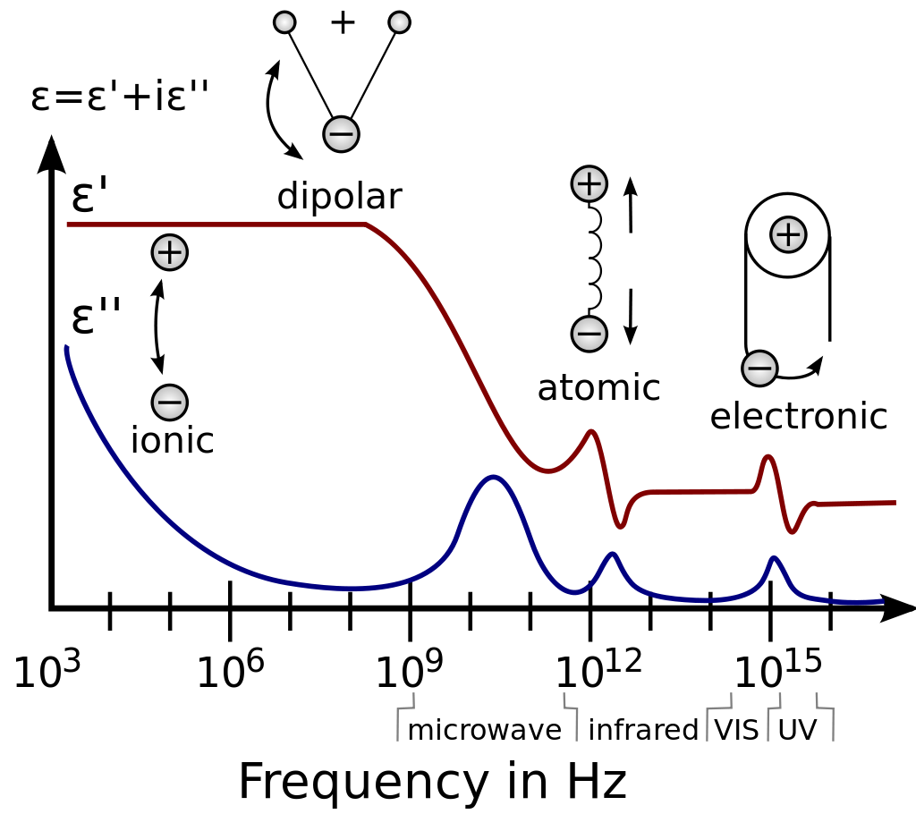
Figure 2.A typical dielectric spectroscopy[2]: dielectric constants are usually imaginary with the real part being permitivity and the imaginary part dielectric loss. The dielectric loss evaluates the asorption of electric energy by a dielectric material subjected to an alternating electric field

Side notes on dielectric spectroscopy: the dielectric constant measured at direct-current condition is called static dielectric, and it contains contributions to polarization from optical and acoustic frequency responces.

We now proceed to derive an expression for the effective dielectric constant \(\bar{\varepsilon}\) from \(\mathbf{P}\). We will use \(\bar{\varepsilon}\) later to calculate the energy of self-trapped electron \(\mathcal{U}\) from which we can further derive the effective mass and size of polaron.

In SI unit the Eq.(4) (with \(\varepsilon_0=1\)) becomes

Because \(\mathbf{D}=\varepsilon\mathbf{E}\), Eq.(11) gives

When a dielectric material is subjected to high-frequency AC electric field,

Let us write that

where \(\varepsilon_{\infty}\) is the high-frequency dielectric constant measured at the AC frequency \(\omega\) right below the ultraviolet resonance. Therefore,

Substracting (13) from (12) gives an expression for \(\mathbf{P}_{acs}\):

Both \(\varepsilon\) and \(\varepsilon_{\infty}\) are experimentally measurable, making the calculation of \(\bar{\varepsilon}\) easy.

The size of the polaron

Accroding to Landau’s model, the charge distribution of a bounded electron is localized within a sphere with radius of \(l_1\). At distances larger than \(l_1\), the field created by the localized electron is Coulombic. Our target in this section is first to calculate the energy of a localized electron with static charge distribution. The total energy will be an expression with \(l_1\) as its parameter. We then find the value of \(l_1\) that minimize the energy. Second, we derive the size of the polaron by considering the dynamics of electron-phonon interactions.

Let us first visualize the field induced by the localized electron in Figure 3 where the charge of our localized electron is uniformly distributed within a sphere with radius of \(l_1\).

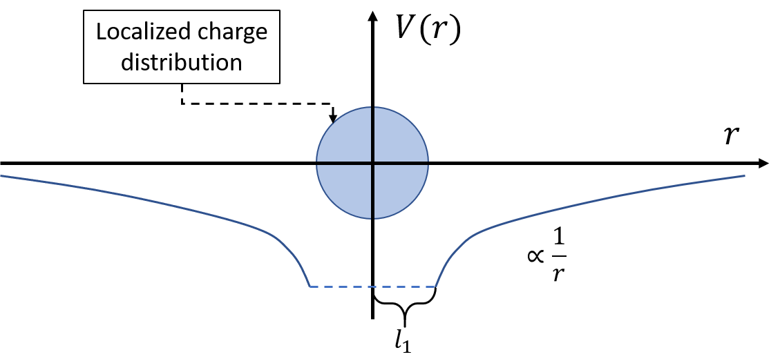
Figure 3. Localized charge distribution assumed in Landau's polaron theory

The Coulombic(potential) energy of our electron friend is of order \(-e^2/\bar{\varepsilon}l_1\) (see Feynman’s derivation here). We use \(\bar{\varepsilon}\) here because we assumed that the polarization induced by the electron is only from acoustic responces. The kinetic energy of the electron is of order \(\hbar^2k^2/2m\) where \(k\) is the characteristic wavenumber of a system with spatial extent of order \(l_1\), i.e. \(k=2\pi/l_1\). Thus the kinetic energy is of order \(4\pi^2\hbar^2/2ml^2_1\), and our estimation of the total energy for the electron in Figure 3, \(\mathcal{U}_1\), is

To find the \(l_1\) that minimze \(\mathcal{U}_1\), we calculate the derivative and find:

and

Substitute (16) into (15) to give

The static charge distribution of the polaron assumed in (15)-(17) is only reasonable when the velocity of electron movements is much faster than that of ions, otherwise the charge distribution would not be able to build up. When the bounded electron moves slower than the propagation of lattice vibration,We need to find the polaron size by studying the dynamic problem of an electron moving with velocity of \(v\) interacting with lattice vibration with frequency of \(\omega\).

If the lattice is vibrating with a frequency \(\omega\), the angular distance travelled by an electron at distance \(d_1\) from an ion (see Figure 4) in a time \(1/\omega\) is just \(v/\omega d_1\). If the angle is small, we have

The limiting value of \(d_1\) for an ion to see an electron as a static charge is of order \(v/\omega\).

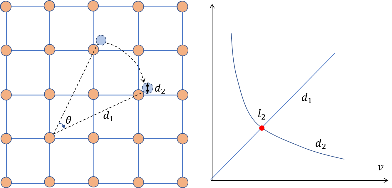
Figure 4. Electron-phonon interaction when the bounded electron moves not so fast, and the ion see the localized electron as a static point charge at d1. The effective radius of the polaron is d2

On the other hand, the effective size of polaron(localized electron) \(d_2\) must not exceed the limiting value of \(d_1\). According to the uncertainty principle,

where the momentum of the electron is \(p=mv\). Therefore,

The right subplot in Figure 4 shows that curves \(d_1(v)\) and \(d_2(v)\) intercept at the distance \(l_2\). For ions outside of the polaron sphere with the radius of \(l_2\), the polaron acts like a static charge. At the intersection,

and

Because the localized electron in Figure 4 moves slower than the electron depiced in Figure 3, the energy of the polaron is just its potential energy, and we have

Effective mass of the polaron

In the previous subsection we discussed the polaron size under two conditions:(1) the fast moving electron with a size of \(l_1\) and (2) the slow moving electron (comparing to the lattice vibration frequency) with a size of \(l_2\). We now propose a simple model, which treated the ions as point charges, to calculate the effective mass of the polaron. In the model the polarization induced by the polaron is represented by the displacements of ions, and the effective mass of the polaron is then derived from the sum of kinetic energies of vibrating ions and mobile polaron.

Let us first derive an expression for the polarization field \(\mathbf{P}\), because by the definition of Eq.(0) \(\mathbf{P}\) is related to the displacement of charge centers. Since we consider ions in the lattice as point charges (e.g. the lattice sketched in Figure 4), the displacements of charge centers (see Figure 1) is ions’ displacements. In Figure 3 we assumed that the induced polarization field is Coulombic outside the localized charge distribution, and is constant inside the confined charge distribution. Use Eq.(14) and the definition of electric field strenth to give:

where \(\mathbf{r}_{e}\) is the bounded electron coordinates, and \(l_i\) could either be \(l_1\) or \(l_2\). The second line in Eq.(22) indicates that \(\rho_b=0\) in the charge distribution of the free electron. The polarization field \(\mathbf{P}\) is again assumed to only contains contributions from acoustic dielectric frequency responces.

We use the assumption of acoustic polarization field again because \(\mathbf{P}_{opt}\) is only important when we have super fast polarons.

According to the definition of Eq.(0), we have

with \(q\) and \(\mathbf{d(r)}\) being ionic charge and relative ionic displacement at arbitrary coodinates, respectively. Substitute (23) into (22), and perform a time derivative to give the kinetic energy of all the displaced ions, \(T_{ion}\), as

\(T_{ion}=\sum_i \frac{1}{2}M\mathbf{\dot{d}_i^2(r)}=\sum_i\frac{1}{2}M\left(\frac{e}{4\pi\bar{\varepsilon}Nq}\frac{\partial}{\partial\mathbf{r}}\frac{\partial}{\partial t}\frac{1}{|\mathbf{r_{e}-r}|}\right)\tag{24}\) where \(M\) is the reduced mass of ion pair. Let \(\mathbf{v}=\dot{\mathbf{r}_e}\) and \(m\) be the velocity and the mass of the bounded electron, the effective mass of the polaron \(m^*\) is then defined as:

We can simplify Eq.(24) by using the following identities of vector derivative:

and

We find that

with

To prove Eq.(26) and (27), we simply expand the vector derivative into its complete form as: \(\frac{d}{d\mathbf{r}}=\frac{d}{dx}\hat{e}_x+\frac{d}{dx}\hat{e}_y+\frac{d}{dx}\hat{e}_z.\)

The sum in Eq.(24) can also be replaced by an integral as follow:

with

and the number density of ion \(N\) is a constant.

Aligning the angle between the vectors \(\mathbf{R}\) and \(\mathbf{v}\) with \(\theta\), we find that

With Eq.(28),(29), and (31) we deduce that

The Eq.(32) is still too bulky to handle, but we can reduce it by using Szigeti relation[3],

As a result, the kinetic energy of vibrating ions is

This expression is independent of the masses of the ions; therefore Landau’s argument that an electron can become self-trapped because the ions are heavy is not valid.[1]

We now see from(25) and (34) that

with \(C_i\) being constants, and the \(\alpha\) is a dimensionless coupling constant and is defined as

We thus obtained a very strong dependence of effective mass on the coupling constants in the case of \(l_i=l_1\). Notice that

When \(\alpha\) is large, \(\left\|\mathcal{U}_{1}\right\|>\left\|\mathcal{U}_{2}\right\| .\) In this case the first type of approximation is better than the second, and the frequency corresponding to \(\left\|\mathcal{U}_{1}\right\|\) is much greater than the oscillation frequency of the polarization(i.e. the polaron moves fast). For large \(\alpha\), we have large \(T_{ion}\) too, indicating the most sytem inertia is carried by the ions outside of the localized electron charge distribution.

Derivation of the Frohlich Hamiltonian

The classical Hamiltonian before quantization

Landau’s phenomenological theory of the polaron triggers his fellow physicists to fromulate a mathematically rigorous Hamiltonian for a system that contains polarons. Like other condensed matter problems, the Hamiltonian for polarons is the center piece for us to understand the energy level distribution of our electron-ion-phonon interactions. One of the most influential formalation is come up with by Frohlich[1] based on quantum field theory. We shall now introduce the derivation of the Frohlich Hamiltonian by borrowing the results from previous sections.

The Frohlich Hamiltonian starts with the assumption of the independence of lattice vibration on the wavevectors, i.e. the group velocity \(d\omega/d\mathbf{k}\) vanishes. As a result, only the longitudinal modes of the polarization \(\mathbf{P}\) is considered (i.e., the infrared dielectric responses,caused by ion displacement[4]). If we use the definition of \(\mathbf{P}\) in Eq.(0) and assumes linear restoring forces to any disturbances in charge distribution(see my blog here for more details), the polarization field can be described by the simple harmonic motion equation:

where \(\mathbf{F}\) is the source term, and the \(\omega\) is the vibrational frequency of induced polarization (or ion displacement). The derivation of Eq.(37) can also be found in my earlier blog here. Because we only care about a slow electron in dielectric material, we can assume that the magnetic field produced by the motion of the electron is negligibly small, and therefore the polarization field must be irrotational:

We now need to figure out what the source term \(\mathbf{F}\) is. Recall that the \(\mathbf{P}\) is related to the displacement field \(\mathbf{D}\) by

Since \(\mathbf{D(r)}\) is the externally applied field, the energy density of \(\mathbf{D-P}\) interaction will be given by \(\mathbf{-D(r) \cdot P(r)}\).

We now make a reasonable guess for the Lagrangian density \(\mathcal{L}\) of our system, from which we can derive a canonical form of Hamiltonian \(H\). The guessing process involves three steps:(1) identify the general field coordinates and their conjugate, (2) form the initial guess by comparing your system with other well-developed system, (3) adjust your Lagrangian density till it satisfies the Euler-Lagrange equation for fields. First, in our case the field coordinates, or the field variables we plug into \(\mathbf{L}\) should be \(\mathbf{P}\) and \(\mathbf{D}\). Second, because \(\mathbf{P}\) is a vector field, and the Lagrangian density \(\mathbf{L}\) in this case should look similar to that for electromagnetic fields, which means that we need a term for the \(\mathbf{P}\) itself, a term for field kinetic energy, and a term for interaction energy. Following the aforementioned logic and using trial-and-error method described in other research[5], we end up with the following Lagrangian density:

where \(\mu\) is a constant needed to be determined. If we take \(\mathbf{P}(\boldsymbol{r})\) as generalized coordinates \(\mathbf{q_{r}}\) at each space point \(\boldsymbol{r}\) then the conjugate generalized momenta \(\mathbf{p_{r}}\) are

We Eq.(39) and (40), the Hamiltonian is then

and

Because the Hamiltonian density \(\mathcal{H}^{\prime}\) is defined as

we have

Combining the equation in (45) we find

Comparing (46) with (37), we see that \(\mathbf{F}=\frac{1}{\mu}\mathbf{D}\). To figure out the format of \(\mu\), we first notice that in the static limit (37) becomes

Since we only consider the longitudinal polarization mode, we have from (12) to (14) that

The Lagrangian density in (39) is not complete as we only consider the fields. But we need to take account for the electron in a polaron-forming system. The Lagrangian of the electrion is just its kinetic energy, i.e.

with \(m^*\) being the Bloch effective mass of the energy. The equation of motion for the electron is then

Because the field \(\mathbf{P}\) is irrotational, we must have another field \(\Phi\) whose gradient gives the field, i.e.

Using \(\Phi\) in our Lagrangian density to find that the complete Lagrangian is

and the complete Hamiltonian is

where \(\mathbf{p}_e=m^*\mathbf{\dot{r}}\),

and

The Eq. (53) used the integration in part at the thir equivalence and droped the surface term because the interaction die out at the boundary. Also we have used the fact that

Note that \(H_{\text {int }}\) depends on the field variables as well as on \(r_{\mathrm{e}}\), although this dependence is not explicitly shown above.

Quantize your Hamiltonian

You probably already noticed that in Eq.(52) I quantized the Hamiltonian of the electron into an operator. Now let us proceed to do the same thing for the rest of the Hamiltonian. Imagine we have a crystalline material whose unit cell has simple cubic volume of \(V=L^3\). The periodic boundary condition (PBC) is applied for the unit cells. Each unit cell contains one extra electron and the Coulombic interaction between two electrons is long-range, so the image of building a material using unit cells and PBC introduce infinite interaction energy, which of course needs to be eliminated during our quantization process.

Let us first expand \(\mathbf{P}\) in terms of space and time as

where PBC on \(V\) requires \(\mathbf{w}=\frac{2 \pi \mathbf{n}}{L},\) with \(\boldsymbol{n}=\left(n_{1}, n_{2}, n_{3}\right) ; n_{j}=0,1,2, \ldots, \infty ; j=1,2,3 .\) The usual procedure to quantize a vector field is to introduce canonical commutation relations between the field coordinates and the corresponding conjugate momenta. In our case the field coordinate is \(\mathbf{P}\) and the conjugate momenta is

The commutation relation between the two should statisfy

which would lead us to define commutation relations for the Fourier components in (54). We also realize that \(\mathbf{P}\) is a real vector field, meaning that its Fourier components \(\mathbf{P_w}\) must be contrained by the following relation

The subsidiary conditions of (56) and (57) meaning that \(\mathbf{P_w}\) are not independent. Since the whole point of doing quantization is to transform the Hamiltonian into a separable format, we should get rid of this dependence among field coordinates. It is found to be more convenient to construct a new field \(\mathbf{B}\) as a linear combination of \(\mathbf{P}\) and \(\mu\dot{\mathbf{P}}\) before we continue our quantization. Thus we define from the canonical transformation[6]:

And therefore,

Because the field \(\mathbf{P}\) is irrotational (its curl is zero), the Fourier components in the expansion of \(\mathbf{B}\), \(\mathbf{B_w}\) should be defined with an unit vector pointing towards the wavevector \(\mathbf{w}\) as:

Using the commutation relation of (56) and Eq.(59) it is easy to show that

From Eq(60) and (61) we have

Insert Eq.(59) with the definitions in Eq.(60) into the field Hamiltonian \(H_F\) in (51) to give

because

We move on to quantize \(H_{int}\) by first noticing that

Since \(\nabla \Phi(r)=4 \pi P(r),\) we see that

Finally, it is instructive to introduce a dimensionless parameter by the following equation:

We then introduce dimensionless electron coordinates, volume parameter, and wave numbers

From Eq.(63),(65) and (52), we obtain

where

This paremeter combination \(\alpha\) is usually referred in research as the Coupling constant.

Conclusion

Now that the quantized Hamiltonian is derived, I need to use it in some simplified models to find the physical properties of modeled systems. Or maybe not since my ultimate goal is to put the Polaron theory in an ab initio calculation framework. Not sure if exactly solved models will help me with that at this point.

References

[1] Kuper, Charles Goethe, and George Danley Whitfield, eds. Polarons and excitons. Plenum Press, 1963.

[2]https://web.archive.org/web/20010307184808/http://www.psrc.usm.edu/mauritz/dilect.html

[3] Szigeti, Bela. “Polarisability and dielectric constant of ionic crystals.” Transactions of the Faraday Society 45 (1949): 155-166.

[4] Chatterjee, Ashok, and Soma Mukhopadhyay. Polarons and Bipolarons: An Introduction. CRC Press, 2018.

[5] Luan, Pi-Gang. “Lagrangian dynamics approach for the derivation of the energy densities of electromagnetic fields in some typical metamaterials with dispersion and loss.” Journal of Physics Communications 2.7 (2018): 075016.

[6] Altland, Alexander, and Ben D. Simons. Condensed matter field theory. Cambridge university press, 2010.