A Pedastrian Approach to Radiation-Matter Interaction-Part III

July 12, 2020

Tags: [basics] [quantum-field-theory]

TL;DR

This blog summarizes the quantized systems introduced in the previous two parts and uses them in the context of radiation-matter interaction.

Bird’s view

We will start with the derivation of the Hamiltonian for a system composed of EM field and free particles. The resulted Hamiltonian will be devided into three parts that describe particles’ energy, EM field energy/radiation energy, and the interaction energy. We then use the Hamiltonian to discuss the examples of light emission from an excited atom, lifetime of excited states, adsorption of photons, photon scattering from free electrons, and some special topics.

Hamiltonian of The EM Field+Paticles System

The system we are interested in here is composed of matters and EM fields, or photons. Usually we would like to think the matter is built up by particles with various masses $m_{i}$ and charges $e_{i}$ . The interactions of these particles are always treated in a form of $V (\dots, x_{i}, \dots)$ . The Coulombic interaction is one example of such interaction,

\begin{matrix} (1.1) & V_{Coulomb} (\dots, x_{i}, \dots, x_{j}, \dots) = \frac{1}{2} \sum_{\binom{i, j}{i \neq j}} \frac{e_{i} e_{j}}{| x_{i} - x_{j} |} . \end{matrix}

Based on the discussions laid out in Part I and II, the Hamiltonian operator for our matter-radiation system can be written as

\begin{matrix} (1.2) & \begin{aligned} \hat{H} = & \sum_{i} \frac{({\hat{p}}_{i} - \frac{e_{1}}{c} \hat{A} (x_{i})) ({\hat{p}}_{i} - \frac{ϵ_{i}}{c} \hat{A} (x_{i}))}{2 m_{i}} + V \\ + \int \frac{\hat{E} \cdot {\hat{E}}^{†} + \hat{B} \cdot {\hat{B}}^{†}}{8 π} d^{3} x \\ = & {\hat{H}}_{mp} + {\hat{H}}_{rad} + {\hat{H}}_{int}, \end{aligned} \end{matrix}

where

\begin{matrix} (1.3) & {\hat{H}}_{mp} = \sum_{i} \frac{{\hat{p}}_{i}^{2}}{2 m_{i}} + V, \end{matrix}

and the “mp” stands for “many particles”. The interaction Hamiltonian is then

\begin{matrix} (1.4) & {\hat{H}}_{int} = \sum_{i} [- \frac{e_{i}}{m_{i} c} {\hat{p}}_{i} \cdot \hat{A} (x_{i}) + \frac{e_{i}^{2}}{2 m_{i} c^{2}} {\hat{A}}^{2} (x_{i})] . \end{matrix}

where we use the Coulomb gauge $\nabla \cdot A = 0$ and Ehrenfest Theorem

\begin{matrix} (1.5) & \begin{array}{l} [x_{i}, F (x, p)] = i ℏ \frac{\partial F}{\partial p_{i}} \\ [p_{i}, G (x, p)] = - i ℏ \frac{\partial G}{\partial x_{i}} \end{array} \end{matrix}

to give $\hat{p} \cdot A + A \cdot \hat{p} = 2 \hat{p} \cdot A$ .

If we only focus on a single particle then (1.5) becomes

{\hat{H}}_{int} = - \frac{e}{m c} \hat{p} \cdot \hat{A} (x) + \frac{e^{2}}{2 m c^{2}} {\hat{A}}^{2} (x) = {\hat{H}}_{i n t}^{'} + {\hat{H}}_{i n t}^{''},

where

\begin{matrix} (1.6) & {\hat{H}}_{int}^{'} = - \frac{e}{m c} \sum_{k, σ} \sqrt{\frac{2 π ℏ c^{2}}{L^{3} ω_{k}}} \hat{p} \cdot ε_{k σ} ({\hat{a}}_{k σ} e^{i k \cdot x} + {\hat{a}}_{k σ}^{†} e^{- i k \cdot x}) \end{matrix}

and

\begin{matrix} (1.7) & \begin{aligned} {\hat{H}}_{int}^{''} = & \frac{e^{2}}{2 m c^{2}} \sum_{k σ} \sum_{k^{'} σ^{'}} (\frac{2 π ℏ c^{2}}{L^{3}}) \frac{ε_{k σ} \cdot ε_{k^{'} σ^{'}}}{{(ω_{k} ω_{k^{'}})}^{\frac{1}{2}}} \\ \times ({\hat{a}}_{k σ} {\hat{a}}_{k^{'} σ^{'}} e^{i (k + k^{'}) \cdot x} + {\hat{a}}_{k σ} {\hat{a}}_{k^{'} σ^{'}}^{†} e^{i (k - k^{'}) \cdot x} \\ + {\hat{a}}_{k σ}^{†} {\hat{a}}_{k^{'} σ^{'}} e^{i (- k + k^{'}) \cdot x} + {\hat{a}}_{k σ}^{†} {\hat{a}}_{k^{'} σ^{'}}^{†} e^{i (- k - k^{'}) \cdot x}) . \end{aligned} \end{matrix}

The interaction energy usually only makes a very small portion of the total energy, so we can treat (1.6) and (1.7) as perturbations. And the undistorbed Hamiltonian, ${\hat{H}}_{m p} + {\hat{H}}_{r a d}$ has the state vectors to be

\begin{matrix} (1.8) & | m p + r a d ⟩ = | m p ⟩ {| \dots n_{k σ} \dots ⟩}_{rad} . \end{matrix}

Several points are worth mentioning regarding ${\hat{H}}_{i n t}$ before we proceed to next section. Because we only have one creation/annhilation in each term of eqn.(1.6), then we conclude that ${\hat{H}}_{i n t}^{'}$ introduces single photon transition. On the other hand, ${\hat{H}}_{i n t}^{''}$ introduces transtions that involve two photons.

Emission of Light From An Excited Atom

In this section we study the transition from an initial particle state, $∣ a_{i} ⟩$ , to a final particle state, $∣ a_{f} ⟩$ by emitting a photon. The the initial and final states for the photon-particle system are then

\begin{matrix} (2.1) & \begin{array}{l} ∣ i ⟩ = | a_{i} ⟩ | \dots, n_{k σ}, \dots ⟩ \\ ∣ f ⟩ = | a_{f} ⟩ | \dots, n_{k σ} + 1, \dots ⟩ \end{array} . \end{matrix}

The corresponding energy levels follow the relation of $E_{i} > E_{f}$ . In Part I we developed Fermi’s golden rule based on perturbation theory, which states that the probability of $i \to f$ transition per unit time is given by

\begin{matrix} (2.2) & \begin{aligned} (\frac{trans. prob.}{time}) = & \frac{2 π}{ℏ} {| M_{fi} |}^{2} δ (E_{f} - E_{i}) \\ M_{fi} = & ⟨ f | {\hat{H}}^{'} | i ⟩ + \sum_{I} \frac{⟨ f | {\hat{H}}^{'} | I ⟩ ⟨ I | {\hat{H}}^{'} | i ⟩}{E_{i} - E_{I} + i η} \\ + \sum_{I, I I} \frac{⟨ f | {\hat{H}}^{'} | I ⟩ ⟨ I | {\hat{H}}^{'} | I I ⟩ ⟨ I I | {\hat{H}}^{'} | i ⟩}{(E_{i} - E_{I} + i η) (E_{i} - E_{II} + i η)} + \dots \end{aligned} \end{matrix}

where ${\hat{H}}^{'}$ is the perturbation Hamiltonian, and $I / I I$ are complete sets of states. The terms other than the first term of $M_{f i}$ are called higher-order transition rate. But here we only consider the fist-order perturbation caused by ${\hat{H}}_{i n t}^{'}$ , i.e.

\begin{matrix} (2.3) & \begin{aligned} ⟨ f | {\hat{H}}_{int}^{'} | i ⟩ \\ = & ⟨ a_{f} | ⟨ \dots, n_{k σ} + 1, \dots | \\ [- \frac{e}{m c} \sum_{k^{'}, σ^{'}} \sqrt{\frac{2 π ℏ c^{2}}{L^{3} ω_{k^{'}}}} \hat{p} \cdot ε_{k^{'} σ^{'}} ({\hat{a}}_{k^{'} σ^{'}} e^{i k^{'} \cdot x} + {\hat{a}}_{k^{'} σ^{'}}^{†} e^{- i k^{'} \cdot x})] \\ ∣ a_{i} ⟩ ∣ \dots, n_{k σ}, \dots ⟩ \\ = & - \frac{e}{m c} \sqrt{\frac{2 π ℏ c^{2}}{L^{3} ω_{k}}} ⟨ a_{f} | \hat{p} \cdot ε_{k σ} e^{- i k \cdot x} | a_{i} ⟩ \\ \times ⟨ \dots, n_{k σ} + 1, \dots | {\hat{a}}_{k σ}^{†} | \dots, n_{k σ}, \dots ⟩ \\ = & - \frac{e}{m c} \sqrt{\frac{2 π ℏ c^{2}}{L^{3} ω_{k}}} ⟨ a_{f} | \hat{p} \cdot ε_{k σ} e^{- i k \cdot x} | a_{i} ⟩ \sqrt{n_{k σ} + 1} . \end{aligned} \end{matrix}

Notice that in the second equivalence above, we only take into account the contribution of the photon with wave vector $k$ and polarization $σ$ . Since the newly emitted photon has an energy of $ℏ ω_{k}$ , eqn.(2.2) to the first order now becomes

\begin{matrix} (2.4) & \begin{aligned} {(\frac{trans. prob.}{time})}_{emission} = & \frac{2 π}{ℏ} {| ⟨ f | {\hat{H}}_{int}^{'} | i ⟩ |}^{2} δ (E_{f} - E_{i}) \\ = & \frac{2 π}{ℏ} {(\frac{e}{m c})}^{2} (\frac{2 π ℏ c^{2}}{L^{3} ω_{k}}) (n_{k σ} + 1) \\ \times {| ⟨ a_{f} | \hat{p} \cdot ε_{k σ} e^{- i k \cdot x} | a_{i} ⟩ |}^{2} \\ \times δ (E_{a_{f}} - E_{a_{i}} + ℏ ω_{k}) . \end{aligned} \end{matrix}

Notice that when there is no photon in our system (i.e. $n_{k σ} = 0$ ), the transition can still happen. This phenomenon is then referred as spontaneous emission. The $1$ in $n_{k σ} + 1$ is the result of commutation rule; this is for the same reason we have $\frac{1}{2}$ in the zero-point energy of EM field[1].

Lifetime of Excited States

Now we consider all the possible $k$ and $σ$ in (2.3) to give an expression for the lifetime of state $i$ , $τ$ , as

\begin{matrix} (3.1) & \begin{aligned} {(\frac{1}{τ})}_{i \to f} = & \frac{2 π}{ℏ} \sum_{k, σ} {| ⟨ f | {\hat{H}}_{int}^{'} | i ⟩ |}^{2} δ (E_{a_{f}} - E_{a_{1}} + ℏ ω_{k}) \\ = & \frac{4 π^{2} e^{2}}{m^{2} L^{3}} \sum_{k, σ} \frac{1}{ω_{k}} {| ⟨ a_{f} | \hat{p} \cdot ε_{k σ} e^{- i k \cdot x} | a_{i} ⟩ |}^{2} \\ \times δ (E_{a_{f}} - E_{a_{1}} + ℏ ω_{k}) . \end{aligned} \end{matrix}

At the limit of $L \to \infty$ , we can replace the summation of wave vector with a integral by

\begin{matrix} (3.2) & \sum_{k} = \frac{L^{3}}{(2 π)^{3}} \int d k . \end{matrix}

The factor in front of the integral is a result from the periodic boundary condition, because PBC dictates that the allowable elements of wavevectors must satisfy the relation of

\begin{matrix} (3.3) & k_{i} L = 2 π n_{i} n_{i} = 0, 1, 2, \dots i = x, y, z . \end{matrix}

Each vector $n = {n_{x}, n_{y}, n_{z}}$ reprents a normal mode of EM field. So the number of normal modes fall into the volume of $Δ n_{x} Δ n_{y} Δ n_{z}$ at $(n_{x}, n_{y}, n_{z})$ is just $L^{3} / (2 π)^{3} Δ k_{x} Δ k_{y} Δ k_{z}$ . At the limit of $L \to \infty$ , (3.2) holds.

Let us now choose the directions of polarization vectors $ε_{k σ}$ so that (3.1) can be largely simplified. If we choose the $ε_{k 1}$ to be a direction perpendicular to $⟨ a_{i} ∣ \hat{p} ∣ a_{f} ⟩$ , and $k$ forms a angle of $θ$ with $⟨ a_{i} ∣ \hat{p} ∣ a_{f} ⟩$ (see Figure 1), we have

\begin{matrix} (3.4) & \begin{aligned} \sum_{σ = 1, 2} {| ⟨ a_{f} | \hat{p} \cdot ε_{k σ} e^{- i k \cdot x} | a_{i} ⟩ |}^{2} & = {| ⟨ a_{f} | \hat{p} \cdot ε_{k_{2}} e^{- i k \cdot x} | a_{i} ⟩ |}^{2} \\ \begin{array}{c} (1.5) \\ = \end{array} {| ε_{k 2} \cdot ⟨ a_{f} | \hat{p} e^{- i k \cdot x} | a_{i} ⟩ |}^{2} \end{aligned} \end{matrix}

where the second equation in (1.5) is used again to swap the place of $ε$ and $k$ . We also notice that the light emitted from an atom has energies of $ℏ ω \approx 10 e V$ , giving that

\begin{aligned} k \cdot x \approx \frac{2 π}{λ} a_{Bohr} & = \frac{ℏ ω}{ℏ c} a_{Bohr} \\ = \frac{10 eV \frac{1}{2} \times 10^{- 8} cm}{1.97 \times 10^{- 5} eV cm} \\ = 2.7 \times 10^{- 3} ≪ 1. \end{aligned}

As a result the exponential factor $e^{- i k \cdot x} \approx 1$ , and eq.(3.4) reduces to

\begin{matrix} (3.5) & \sum_{σ = 1, 2} {| ⟨ a_{f} | \hat{p} \cdot ε_{k σ} e^{- i k \cdot x} | a_{i} ⟩ |}^{2} \approx {| ε_{k 2} \cdot ⟨ a_{f} | \hat{p} | a_{i} ⟩ |}^{2} . \end{matrix}

Eq.(3.5) is often referred as dipole approximation for the reasons we will discuss later. Similarly, we also have magnetic dipole approximation with $e^{- i k \cdot x} \approx 1 - i k \cdot x$ , and electric quadrupole approximation with $e^{- i k \cdot x} \approx 1 - i k \cdot x - \frac{1}{2} (k \cdot x)^{2} .$

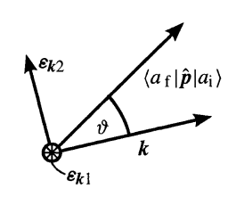
Figure 1. The choice of one of the polarization vectors. The angle theta represents the polar angle in k-space.

From figure 1 it is easy to get

| | ε_{k 2} | | ⟨ a_{f} | \hat{p} | a_{i} ⟩ {| \cos (90^{\circ} - ϑ) |}^{2} = {| ⟨ a_{f} | \hat{p} | a_{i} ⟩ |}^{2} \sin^{2} ϑ,

and finally

\begin{matrix} (3.6) & {(\frac{1}{τ})}_{i \to f} = \frac{e^{2}}{2 π m^{2}} \int d^{3} k \frac{1}{ω_{k}} {| ⟨ a_{f} | \hat{p} | a_{i} ⟩ |}^{2} \sin^{2} ϑ δ (E_{a_{f}} - E_{a_{i}} + ℏ ω_{k}) . \end{matrix}

If we use spherical coordinate to do the integral and let $ω_{f i}$ be the photon frequence that conserve energy, then

\begin{matrix} (3.7) & \begin{aligned} {(\frac{1}{τ})}_{i \to f} = & \frac{e^{2} 2 π}{2 π m^{2} c^{3}} \int d ω_{k} ω_{k} {| ⟨ a_{f} | \hat{p} | a_{i} ⟩ |}^{2} \\ \times δ (E_{a_{f}} - E_{a_{1}} + ℏ ω_{k}) \int_{0}^{π} \sin^{3} ϑ d ϑ \\ = & \frac{4}{3} \frac{e^{2}}{m^{2} c^{3} ℏ} ω_{fi} {| ⟨ a_{f} | \hat{p} | a_{i} ⟩ |}^{2} . \end{aligned} \end{matrix}

The matrix element $⟨ a_{f} ∣ \hat{p} ∣ a_{i} ⟩$ can be cast in another form, i.e.

\begin{matrix} (3.8) & \begin{aligned} ⟨ a_{f} | \hat{p} | a_{i} ⟩ & = ⟨ a_{f} | m \frac{d \hat{x}}{d t} | a_{i} ⟩ \\ = - \frac{i}{ℏ} m ⟨ a_{f} | \hat{x} {\hat{H}}_{mp} - {\hat{H}}_{mp} \hat{x} | a_{i} ⟩ \\ = - \frac{i m}{ℏ} (E_{a_{i}} - E_{a_{f}}) ⟨ a_{f} | \hat{x} | a_{i} ⟩ \\ = - i m ω_{fi} ⟨ a_{f} | \hat{x} | a_{i} ⟩ . \end{aligned} \end{matrix}

The Heisenberg’s equation of motion is used at the second equivalence, that is,

\frac{d \hat{x}}{d t} = - \frac{i}{ℏ} [\hat{x}, {\hat{H}}_{mp}]

Applying the trick in (3.8) we recognize that the momentum matrix element $e ⟨ a_{f} ∣ \hat{p} ∣ a_{i} ⟩$ can be expressed as a matrix element of the dipole operator $e \hat{x}$ . By now the designations dipole approximation and dipole radiation introduced earlier should have become clear.

The Hamiltonian for interaction btw the electron Spin and the EM field

Up to this point we neglect the interaction btw particle spin and EM field. To add it in our Hamiltonian, we first realize that the interaction energy of a magnetic momentum $μ$ and a magnetic field $B$ is just

\begin{matrix} (3.9) & H^{'''} = - μ \cdot B \end{matrix}

where $μ = (e ℏ / 2 m c) σ$ . Since $B = \nabla \times A$ we can quantize (3.9) as

{\hat{H}}^{'''} = - \frac{i e ℏ}{2 m c} \sum_{k, σ} N_{k} σ \cdot (\hat{k} \times ε_{k σ}) [{\hat{a}}_{k σ} e^{i k \cdot r} + {\hat{a}}_{k σ}^{†} e^{- i k \cdot r}],

where $\hat{k} = - i \nabla$ . Acting $\hat{k}$ on exponential factors gives

\begin{matrix} (3.10) & {\hat{H}}^{'''} = - \frac{i e ℏ}{2 m c} \sum_{k, σ} N_{k} σ \cdot (k \times ε_{k σ}) [{\hat{a}}_{k σ} e^{i k \cdot r} - {\hat{a}}_{k σ}^{†} e^{- i k \cdot r}] . \end{matrix}

Adsorption of Photons

The adsorption process is exact opposite to the emission process. Thus, the initial and final states of the phonon+particle system are

\begin{matrix} (4.1) & \begin{array}{l} | i ⟩ = | a_{i} ⟩ | \dots, n_{k σ}, \dots ⟩, \\ ∣ f ⟩ = | a_{f} ⟩ | \dots, n_{k σ} - 1, \dots ⟩ . \end{array} \end{matrix}

and the matrix element of ${\hat{H}}_{i n t}^{'}$ is

\begin{matrix} (4.2) & \begin{aligned} ⟨ f | {\hat{H}}_{int}^{'} | i ⟩ = & ⟨ a_{f} | ⟨ \dots, n_{k σ} - 1, \dots | \\ \times (- \frac{e}{m c}) \sum_{k, σ} \sqrt{\frac{2 π ℏ c^{2}}{L^{3} ω_{k}}} \hat{p} \cdot ε_{k σ} ({\hat{a}}_{k σ} e^{i k^{'} \cdot x} + {\hat{a}}_{k σ}^{†} e^{- i k^{'} \cdot x}) \\ \times | a_{i} ⟩ | \dots, n_{k σ}, \dots ⟩ \\ = & - \frac{e}{m c} \sqrt{\frac{2 π ℏ c^{2}}{L^{3} ω_{k}}} ⟨ a_{f} | \hat{p} \cdot ε_{k σ} e^{i k \cdot x} | a_{i} ⟩ \\ \times ⟨ \dots, n_{k σ} - 1, \dots | {\hat{a}}_{k σ} | \dots, n_{k σ}, \dots ⟩ \\ = & - \frac{e}{m c} \sqrt{\frac{2 π ℏ c^{2}}{L^{3} ω_{k}}} ⟨ a_{f} | \hat{p} \cdot ε_{k σ} e^{i k \cdot x} | a_{i} ⟩ \sqrt{n_{k σ}} \end{aligned} \end{matrix}

where we once again only consider one photon with wave vector $k$ and polarization $σ$ . The probability of transition per unit time is then

\begin{matrix} (4.3) & \begin{aligned} {(\frac{trans. prob.}{time})}_{absorption} = & \frac{2 π}{ℏ} {(\frac{e}{m c})}^{2} (\frac{2 π ℏ c^{2}}{L^{3} ω_{k}}) n_{k σ} \\ \times {| ⟨ a_{f} | \hat{p} \cdot ε_{k σ} e^{i k \cdot x} | a_{i} ⟩ |}^{2} δ (E_{f} - E_{i}) \end{aligned} \end{matrix}

with

\begin{array}{l} E_{f} = E_{a_{f}} + (n_{k σ} - 1) ℏ ω_{k σ} \\ E_{i} = E_{a_{i}} + n_{k σ} ℏ ω_{k σ} . \end{array}

If we make use of the relation

⟨ a_{f} | \hat{p} \cdot ε_{k σ} e^{i k \cdot x} | a_{i} ⟩ = {⟨ a_{i} | \hat{p} \cdot ε_{k σ} e^{- i k \cdot x} | a_{f} ⟩}^{*}

eqn.(4.3) becomes

\begin{matrix} (4.4) & \begin{array}{l} (\frac{trans. prob.}{time}) \\ \begin{matrix} = \frac{2 π}{ℏ} {(\frac{e}{m c})}^{2} (\frac{2 π ℏ c^{2}}{L^{3} ω_{k}}) n_{k σ} {| ⟨ a_{i} | \hat{p} \cdot ε_{k σ} e^{- i k \cdot x} | a_{f} ⟩ |}^{2} \\ \times δ (E_{a_{i}} + ℏ ω_{k σ} - E_{a_{f}}) \end{matrix} \end{array} \end{matrix}

which is similar to eqn.(2.4) with $n_{k σ} + 1$ replaced by $n_{k σ}$ . We will now calculate the cross section $σ_{i \to f} (k σ)$ for the absorption of a photon with momentum $ℏ k$ and polarization $σ .$ It is defined as the transition probability per unit time for the absorption of a photon divided by the incoming photon flux $j_{photon}$ ,

\begin{matrix} (4.5) & j_{photon} = \frac{n_{k σ}}{L^{3}} c . \end{matrix}

We call $σ_{i \to f}$ “cross section” because it has an unit of area. The definition yields that

\begin{matrix} (4.6) & \begin{aligned} σ_{i \to f} (k σ) = & \frac{4 π^{2} e^{2}}{m^{2} ω_{k} c} {| ⟨ a_{f} | \hat{p} \cdot ε_{k σ} e^{i k \cdot x} | a_{i} ⟩ |}^{2} \\ \times δ (E_{a_{i}} + ℏ ω_{k} - E_{a_{f}}) . \end{aligned} \end{matrix}

Photon Scattering from Free Electrons

In this section we will first prove that free paritlce in vacuum cannot radiate any photon by borrowing the concept of 4-momentum from special relativity. This phenomenon is a result of using eigenstates of free particles. We then study the scattering between a photon and a free electron.

The Hamiltonian for a free particle in vacuum is simply

\begin{matrix} (5.1) & \hat{H} = \frac{{\hat{p}}^{2}}{2 m}, \end{matrix}

with normalized eigenstates $∣ q ⟩$ being

\begin{matrix} (5.2) & ⟨ x ∣ q ⟩ = ψ_{q} (x) = \frac{1}{\sqrt{L^{3}}} e^{i q \cdot x} . \end{matrix}

At first, we consider the process of a free electron absorbing a photon. The initial and final states are given by

\begin{array}{l} | i ⟩ = | q_{i} ⟩ | \dots, n_{k σ}, \dots ⟩ \\ | f ⟩ = | q_{f} ⟩ | \dots, n_{k σ} - 1, \dots ⟩ \end{array}

and from previous section we also have

\begin{matrix} (5.3) & \begin{aligned} ⟨ f | {\hat{H}}_{int}^{'} | i ⟩ = & ⟨ q_{f} | ⟨ \dots, n_{k σ} - 1, \dots | (- \frac{e}{m c}) \hat{p} \cdot ε_{k σ} \sqrt{\frac{2 π ℏ c}{L^{3} ω_{k}}} \\ \times ({\hat{a}}_{k σ} e^{i k \cdot x} + {\hat{a}}_{k σ}^{†} e^{- i k \cdot x}) | q_{i} ⟩ | \dots, n_{k σ}, \dots ⟩ \\ = & - \frac{e}{m c} \sqrt{\frac{2 π ℏ c}{L^{3} ω_{k}}} ⟨ q_{f} | \hat{p} \cdot ε_{k σ} e^{i k \cdot x} | q_{i} ⟩ \sqrt{n_{k σ}} \\ = & - \frac{e}{m c} \sqrt{\frac{2 π ℏ c}{L^{3} ω_{k}}} (- q_{f} \cdot ε_{k σ}) \sqrt{n_{k σ}} \\ \times \int_{L^{3}} \frac{e^{- i q_{f} \cdot x}}{L^{3 / 2}} e^{i k \cdot x} \frac{e^{i q \cdot x}}{L^{3 / 2}} d^{3} x . \end{aligned} \end{matrix}

Notice that the third equivalence is right because the exponential factor in the “sandwhich” is a constant and the momentum operator $\hat{p}$ was applied to the $∣ q_{i} ⟩$ state directly. The integral in (5.3) yields a delta function,i.e.

\begin{matrix} (5.4) & \int_{L^{3}} \frac{e^{- i q_{f} \cdot x}}{\sqrt{L^{3}}} \frac{e^{i (q_{i} + k) \cdot x}}{\sqrt{L^{3}}} d^{3} x = δ_{q_{f}, q_{i} + k} \end{matrix}

which indicates the conservation of momentum,

\begin{matrix} (5.5) & ℏ q_{f} = ℏ q_{i} + ℏ k . \end{matrix}

Meanwhile, we also have to satisfy the energy conservation law, which gives

\begin{matrix} (5.6) & E_{f} = E_{i} or \frac{{(ℏ q_{f})}^{2}}{2 m} = ℏ ω_{k} + \frac{{(ℏ q_{i})}^{2}}{2 m} . \end{matrix}

Now we are about to see that we cannot satisfy (5.5) and (5.6) in the case of free particle in vacuum. From special relativity the 4-momentum vector for a paticle, $P_{a}^{μ}$ , and a photon, $P_{γ}^{μ}$ are

\begin{matrix} (5.7) & P_{a}^{μ} = (\frac{E}{c}, p, 0, 0), \end{matrix}

and

\begin{matrix} (5.8) & P_{γ}^{μ} = (E_{γ} / c, \frac{E v_{x}}{c^{2}}, \frac{E v_{y}}{c^{2}}, \frac{E v_{z}}{c^{2}}) . \end{matrix}

Notice that (5.8) gives the massless photon as

P_{γ}^{μ} \cdot P_{μ, γ} = m^{2} = 0.

where the natural unit is used. Eq.(5.7) alignes the move direction of the particle to x-axis. Let us assume the emitted photon propagates at a direction forming a $θ$ angle with x-axis, that is

\begin{matrix} (5.9) & P_{γ}^{μ} = \frac{E}{c} (1, c o s θ, s i n θ, 0) . \end{matrix}

The 4-momentum of new particle is then

\begin{matrix} (5.10) & P_{a^{'}}^{μ} = (\frac{E^{'}}{c}, p^{'}) . \end{matrix}

and $P_{a^{'}}^{μ} = P_{a}^{μ} - P_{γ}^{μ} .$

If we apply the Lorentz invariance and calculate the 4-vector products using Minkowski metric, we have

\begin{matrix} (5.12) & \begin{aligned} P_{a}^{' μ} \cdot P_{a, μ}^{'} & = (P_{a}^{μ} - P_{γ}^{μ}) \cdot (P_{a, μ} - P_{γ, μ}) \\ m_{a}^{2} & = m_{a}^{2} + m_{γ}^{2} - 2 P_{a}^{μ} P_{γ, μ} \end{aligned} . \end{matrix}

Because $m_{γ} = 0$ eqn.(5.12) is found to be

\begin{matrix} (5.13) & P_{a}^{μ} \cdot P_{γ, μ} = \frac{E \cdot E_{γ}}{c^{2}} - \frac{p \cdot E_{γ}}{c} \cos θ = E_{γ} (E - c p c o s θ) = 0 \end{matrix}

where we recover the light speed from the natural unit. Remember the identity in special relativity

\begin{matrix} (5.14) & E = \sqrt{m^{2} c^{4} + c^{2} p^{2}} \to E > p c \end{matrix}

we finally conclude from (5.13) that $E_{γ} = 0$ , i.e., no photon emission is possible. In a similar way, one can also prove that the free particle in vacuum does not absorb photon too.

We can also draw the conclusion that processes of first order caused by ${\hat{H}}_{int}^{'}$ do not exist. As a consequence we investigate now the processes of first order with ${\hat{H}}_{int}^{''} .$ for the free particles. This part of the interaction contains terms of the form ${\hat{a}}_{k σ}^{†} {\hat{a}}_{k^{'} σ^{'}} .$ Obviously, they describe processes that can be shown in the following sketch.

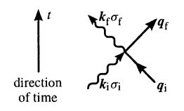
Figure 2. Sketch of a two-photon process in k-space

In figure 2 the wiggly and solid lines represent photons and particles, respectively. The initial and final states described above are then

\begin{matrix} (5.15) & \begin{array}{l} | i ⟩ = | q_{i} ⟩ | \dots, n_{k_{1} σ_{1}}, \dots, n_{k_{f} σ_{t}}, \dots ⟩ \\ | f ⟩ = | q_{f} ⟩ | \dots, n_{k_{i} σ_{i}} - 1, \dots, n_{k_{f} σ_{f}} + 1, \dots ⟩ . \end{array} \end{matrix}

The transition probability per unit time is thus,

\begin{matrix} (5.16) & \begin{aligned} (\frac{trans. prob.}{time}) & = \frac{2 π}{ℏ} {(\frac{e^{2}}{2 m c^{2}})}^{2} {(\frac{2 π ℏ c^{2}}{L^{3}})}^{2} \frac{{| ε_{k_{1} σ_{f}} \cdot ε_{k_{1} σ_{1}} |}^{2}}{ω_{k_{1}} ω_{k_{f}}} \\ \times | ⟨ q_{f} | ⟨ \dots, n_{k_{1} σ_{1}} - 1, \dots, n_{k_{f} σ_{f}} + 1, \dots | \\ \times ({\hat{a}}_{k_{i} σ_{i}} {\hat{a}}_{k_{f} σ_{f}}^{†} e^{i (k_{i} - k_{f}) \cdot x} + {\hat{a}}_{k_{f} σ_{f}}^{†} {\hat{a}}_{k_{i} σ_{i}} e^{i (k_{i} - k_{f}) \cdot x}) \\ \times {| q_{i} ⟩ | \dots, n_{k_{i} σ_{i}}, \dots, n_{k_{f} σ_{f}}, \dots ⟩ |}^{2} \\ \times δ (ℏ ω_{i} + \frac{{(ℏ q_{i})}^{2}}{2 m} - ℏ ω_{f} - \frac{{(ℏ q_{f})}^{2}}{2 m}) \end{aligned} \end{matrix}

Applying the creation and annhilation operators to the states gives

\begin{matrix} (5.17) & \begin{aligned} {(\frac{trans. prob.}{time})}_{photon scattering} \\ = \frac{8 π}{ℏ} {(\frac{e^{2}}{2 m c^{2}})}^{2} {(\frac{2 π ℏ c^{2}}{L^{3}})}^{2} \frac{{| ε_{k_{1} σ_{f}} \cdot ε_{k_{1} σ_{1}} |}^{2}}{ω_{k_{1}} ω_{k_{1}}} \\ \times {| ⟨ q_{f} | e^{i (k_{i} - k_{f}) \cdot x} | q_{i} ⟩ |}^{2} n_{k_{i} σ_{i}} (n_{k_{f} σ_{f}} + 1) \\ \times δ (ℏ ω_{k_{i}} + \frac{{(ℏ q_{i})}^{2}}{2 m} - ℏ ω_{k_{f}} - \frac{{(ℏ q_{f})}^{2}}{2 m}) \end{aligned} \end{matrix}

The matrix element in the squred bracket is then

\begin{aligned} ⟨ q_{f} | e^{i (k_{1} - k_{f}) \cdot x} | q_{i} ⟩ & = \int d^{3} x \frac{e^{- i (q_{f} + k_{f}) \cdot x}}{\sqrt{L^{3}}} \frac{e^{i (q_{i} + k_{i}) \cdot x}}{\sqrt{L^{3}}} \\ = δ_{q_{f} + k_{t}, k_{i} + q_{l}} \end{aligned}

which indicates the conservation of momenta.

Natural linewidth and self-energy

So far all the transition probability expressions from previous sections have $δ -$ functions to satisfy the momentum/energy conservation. However, the photon emitting from a particle corresponds to a wave of finite length and duration. According to the Heisenberg’s uncertainty principle, there must be uncertainty in particle’s energy that is related to the lifetime of excited states, i.e. $Δ E \geq ℏ / τ$ . Therefore, the photon emission spectrum from a particle must be made of lines with finide width rather than a spectrum of infinite peaks of $δ -$ function. This section shows a way to correct such error.

Here we employ a method that is similar to what we have seen in the coherence state section of Part II blog, that is, writing the eigenstates of EM+particle system $∣ ψ ⟩$ as a linear combination of unperturbed states $∣ ϕ_{n} ⟩$ ,

\begin{matrix} (6.1) & | ψ ⟩ = \sum_{n} c_{n} (t) \exp (- \frac{i E_{n}}{ℏ} t) | ϕ_{n} ⟩, \end{matrix}

where

\begin{matrix} (6.2) & ({\hat{H}}_{m p} + {\hat{H}}_{r a d}) | ϕ_{n} ⟩ = E_{n} | ϕ_{n} ⟩ . \end{matrix}

Using (6.1) and (6.2) in the time-dependent Schrodinger equation gives a system of coupled equations

\begin{matrix} (6.3) & \frac{d c_{m} (t)}{d t} = - \frac{i}{ℏ} \sum_{n} c_{n} (t) ⟨ ϕ_{m} | {\hat{H}}_{int} | ϕ_{n} ⟩ \exp (\frac{i (E_{m} - E_{n}) t}{ℏ}) . \end{matrix}

We now let $c_{i 0}$ to be the amplitude of the initial state with no photon, while $c_{f k σ}$ to be the possible final states’ amplitudes. Then (6.3) reads

\begin{matrix} (6.4) & \begin{aligned} \frac{d c_{i 0}}{d t} & = - \frac{i}{ℏ} \sum_{k σ} ⟨ i 0 | {\hat{H}}_{i n t} | f k σ ⟩ \exp (\frac{i}{ℏ} (E_{i} - E_{f} - ℏ ω_{k}) t) c_{f k σ}, \\ \frac{d c_{f k σ}}{d t} & = - \frac{i}{ℏ} ⟨ f k σ | {\hat{H}}_{int} | i 0 ⟩ \exp (- \frac{i}{ℏ} (E_{i} - E_{f} - ℏ ω_{k}) t) c_{i 0} . \end{aligned} \end{matrix}

Note that the first equation still contains a sum because the initial state could decay into many different states, while each final state has only one initial state from which it is derived. Hence the second equation of (6.4) has no summation. Now we make the ansatz of

\begin{matrix} (6.5) & c_{i 0} (t) = \exp (- \frac{i}{ℏ} Δ E_{i} t) \end{matrix}

where $Δ E_{i}$ is a constant needed to be determined. Use(6.5) and integrate the second equation of (6.4) from 0 to $t$ to get

\begin{matrix} (6.6) & c_{f k σ} (t) = ⟨ f k σ | {\hat{H}}_{int} | i 0 ⟩ \frac{\exp [- \frac{i}{ℏ} (E_{i} + Δ E_{i} - E_{f} - ℏ ω_{k}) t] - 1}{E_{i} + Δ E_{i} - E_{f} - ℏ ω_{k}} . \end{matrix}

We now determine $Δ E_{i}$ so that the first equation of (6.4) is satisfied too. Using (6.5) and (6.6) in the first equation of (6.4) we find

\begin{aligned} - \frac{i}{ℏ} Δ E_{i} \exp (- \frac{i}{ℏ} Δ E_{i} t) \\ = & - \frac{i}{ℏ} \sum_{k σ} ⟨ i 0 | {\hat{H}}_{int} | f k σ ⟩ ⟨ f k σ | {\hat{H}}_{int} | i 0 ⟩ \\ \times \frac{\exp [- \frac{i}{ℏ} (E_{i} + Δ E_{i} - E_{f} - ℏ ω_{k}) t] - 1}{E_{i} + Δ E_{i} - E_{f} - ℏ ω_{k}} \exp (\frac{i}{ℏ} (E_{i} - E_{f} - ℏ ω_{k}) t) \\ = & - \frac{i}{ℏ} \sum_{k σ} {| ⟨ f k σ | {\hat{H}}_{int} | i 0 ⟩ |}^{2} \frac{1 - \exp [\frac{i}{ℏ} (E_{i} + Δ E_{i} - E_{f} - ℏ ω_{k}) t]}{E_{i} + Δ E_{i} - E_{f} - ℏ ω_{k}} \\ \times \exp (- \frac{i}{ℏ} (E_{i} + Δ E_{i} - E_{f} - ℏ ω_{k}) t + \frac{i}{ℏ} (E_{i} + Δ E_{i} - E_{f} - ℏ ω_{k}) t) \end{aligned}

Dividing both side by $(- i / ℏ) \exp (- \frac{i}{ℏ} Δ E_{i} t)$ results in

\begin{matrix} (6.7) & \begin{aligned} Δ E_{i} = & \sum_{k σ} {| ⟨ f k σ | {\hat{H}}_{int} | i 0 ⟩ |}^{2} \\ \times (\frac{1 - \exp (\frac{i}{ℏ} (E_{i} + Δ E_{i} - E_{f} - ℏ ω_{k}) t)}{E_{i} + Δ E_{i} - E_{f} - ℏ ω_{k}}) . \end{aligned} \end{matrix}

To further simplify (6.7) we ask mathmatician for help. Here we need the Plemlj’s Formula,

\begin{matrix} (6.8) & lim_{t \to \infty} (\frac{1 - e^{i x t}}{x}) = P (\frac{1}{x}) - i π δ (x), \end{matrix}

and turn (6.7) into

\begin{matrix} (6.9) & \begin{aligned} Δ E_{i} = & \sum_{k σ} \frac{{| ⟨ f k σ | {\hat{H}}_{int}^{'} | i 0 ⟩ |}^{2}}{E_{i} + Δ E_{i} - E_{f} - ℏ ω_{k}} \\ - i π \sum_{k σ} {| ⟨ f k σ | {\hat{H}}_{int}^{'} | i 0 ⟩ |}^{2} δ (E_{i} + Δ E_{i} - E_{f} - ℏ ω_{k}) . \end{aligned} \end{matrix}

Hence, $Δ E_{i}$ is complex-valued. We write the real part and imaginary part separately to find

\begin{matrix} (6.10) & \begin{array}{l} ℜ (Δ E_{i}) = \sum_{k, σ} \frac{{| ⟨ f k σ | {\hat{H}}_{int}^{'} | i 0 ⟩ |}^{2}}{E_{i} - E_{f} - ℏ ω_{k}}, \\ ℑ (Δ E_{i}) = - π \sum_{k, σ} {| ⟨ f k σ | {\hat{H}}_{int}^{'} | i 0 ⟩ |}^{2} δ (E_{i} - E_{f} - ℏ ω_{k}) . \end{array} \end{matrix}

If there are many final states that the particle could stay after the decay, we need to sum over those states too, and (6.10) is modified into

\begin{matrix} (6.11a,b) & \begin{array}{l} ℜ (Δ E_{i}) = \sum_{k, σ} \sum_{f} \frac{{| ⟨ f k σ | {\hat{H}}_{int}^{'} | i 0 ⟩ |}^{2}}{E_{i} - E_{f} - ℏ ω_{k}}, \\ ℑ (Δ E_{i}) = - {π \sum_{k, σ} \sum_{f} | ⟨ f k σ | {\hat{H}}_{int}^{'} | i 0 ⟩ | |}^{2} δ (E_{i} - E_{f} - ℏ ω_{k}) . \end{array} \end{matrix}

The summation in (6.11a) is unrestricted, meaning that the final state could not fulfill the energy conservation. This phenomenon is called virtual process where the particle is understood as a combination of a bare particle and virtual photon cloud. This phenomenon also indicates that quantum field theory is plagued by the infinities, and the solution to such problem is the renormalization group.

On the other hand (6.11b) can be recasted into a form of

\begin{matrix} (6.12) & - \frac{2}{ℏ} ℑ (Δ E_{i}) = \sum_{k σ} \sum_{f} \frac{2 π}{ℏ} {| ⟨ f k σ | {\hat{H}}_{int}^{'} | i 0 ⟩ |}^{2} δ (E_{i} - E_{f} - ℏ ω) . \end{matrix}

Comparing (6.12) with (3.1) we can tell that the imaginary part of $Δ E_{i}$ is directly related to the reciprocal lifetime of initial state, i.e.

\begin{matrix} (6.13) & \frac{1}{τ_{i}} = γ_{i} = - \frac{2}{ℏ} ℑ (Δ E_{i}) . \end{matrix}

Thus, the initial particle state $∣ a_{i} ⟩$ decays with lifetime $τ .$ On the same footing the state obtains a level shift $ℜ (Δ E),$ which results from the emission and reabsorption of (virtual) photons.

With the calculated $Δ E_{i}$ the probability amplitude of finding a final state to be $f$ with wave vector $k$ and polarization $σ$ is then

\begin{matrix} (6.14) & c_{f k σ} (t) = ⟨ f k σ | {\hat{H}}_{int}^{'} | i 0 ⟩ \frac{\exp (- \frac{i}{ℏ} (E_{i} + ℜ (Δ E_{i}) - ℏ ω_{k}) t) \exp (- γ_{i} t / 2) - 1}{E_{i} + ℜ (Δ E_{i}) - E_{f} - ℏ ω_{k} + (i / 2) ℏ γ_{i}}, \end{matrix}

from which the probability of finding a specific final state after a long time is

\begin{matrix} (6.15) & \begin{aligned} lim_{t \to \infty} {| c_{f k σ} |}^{2} = & {| ⟨ f k σ | {\hat{H}}_{int}^{'} | i 0 ⟩ |}^{2} \\ \times \frac{1}{{(E_{i} + ℜ (Δ E_{i}) - E_{f} - ℏ ω_{k})}^{2} + ℏ^{2} γ_{i}^{2} / 4} . \end{aligned} \end{matrix}

Eq.(6.15) reflects the intensity distribution of the emitted line: The spectral line has a Breit-Wigner distribution with center $ℏ ω_{k} = E_{i} + ℜ (Δ E_{i}) - E_{f}$ and half-width $ℏ γ_{i};$ . Because of the self-energy of the electron, emission and reabsorption of photons results in the spectral line being shifted by $ℜ (Δ E_{i}) .$

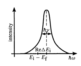
Figure 3. Breit-Wigner form of the spectral line

Conclusion

Let us call a stop to this radiation-matter interaction journey. This is the first time I write a series of blogs for quantum field theory basics. There are still so many aspects we can talk about this amazing starting point towards the general application of QFT. Along the way I learned that a good theory always starts from a basic equation that is not going to breakdown no matter what. To derive useful conclusions from a theory we have to keep coming back to the basics to assure ourselves that the final results are not artificial but can be interpreted using real-world phenomena. I also restrained myself to only focus on the aspects that might be helpful for me to better understand the polaron theory, hopefully more about polaron theory will be finished after my prelim exam.

References

[1] Greiner, Walter. Quantum Mechanics: Special Chapters. Berlin-New York: Springer, 1998.