Electrons in Periodic Potentials (Tight-binding)
May 28, 2020
Background
We have discussed what an eigenstate might look like mathematically for an electron in periodic potential using Bloch’s theorem. In this blog we move forward with a closer look on the operators that could be applied to electron eigenstates. After an introduction to two important evolution operators, we will use the information we have so far to examine the energy band structure of electrons in a simple case: tight-binding model.
Time and space evolution operator
Time evolution operator
Quantum mechanics has three mathematical formulation: Schrodinger’s Picture (SP), Heisenberg’s Picture (HP), and Interaction Picture(IP). In SP the operators applied to quantum states are time-invariant but the states are time-dependent. In HP the condition is reversed, and it only contrasts with SP by a basis transformation. To see this, imagine you have an operator \(A\) in SP, and its expectation value is:
\[\langle\phi(t)|A|\phi(t)\rangle\]Note that the quantum state here is time-dependent. Now we make a base transformation on \(A\) using a “time-evolution operator”, \(U(t)\) as:
\[A(t)=U^{\dagger}(t)AU(t).\]If we apply this time-evolution operator on quantum state \(\|\phi(0)\rangle\) we have \(U(t)\|\phi(0)\rangle=\|\phi(t)\rangle\). Comparing this to the expectation value in SP we should now appreciate the argument of basis transformation between SP and HP, because:
\[\langle\phi(t)|A|\phi(t)\rangle_{SP}=\langle\phi(0)|U^{\dagger}(t)AU(t)|\phi(0)\rangle=\langle\phi|A(t)|\phi\rangle_{HP}.\]The Schrodinger equation for the time-evolution operator is:
\[\frac{i\hbar\partial}{\partial t}U(t)=HU(t)\]When the Hamiltonian is not time-dependent we can write the time-evolution operator as:
\[U(t)=e^{-iHt/\hbar}\tag{1}\]With Eq. (1) we can now define the interaction picture where both quantum state and operators are time-dependent. First, the Hamiltonian from SP is divided into two parts: time-independent part \(H_0\) and time-dependent part \(H_I\). Sometimes, we found it makes more sense to divide it into solvable part and unsolvable part. The quantum state in IP now becomes:
\[|\phi(t)\rangle_{IP}=e^{iH_0t/\hbar}|\phi(t)\rangle_{SP}\]and the operators are similar to those in HP:
\[A_{IP}(t)=e^{iH_0t/\hbar}Ae^{-iH_0t/\hbar}\]For the Hamiltonian operator itself, the time-independent/solvable part \(H_{0,IP}\) is:
\[H_{0,IP}=e^{iH_0t/\hbar}H_{0}e^{-iH_0t/\hbar}=H_0\]and the time-dependent/unsolvable part in IP is:
\[H_{1,IP}=e^{iH_0t/\hbar}H_1e^{-iH_0t/\hbar}\]Space evolution operator
Just like the time evolution, our quantum states can evolve in the real space also. Let’s say we have a state at coordinate x, \(\|x\rangle\), and we apply a space evolution operator \(\hat{T}\) on it to change its coordinate by \(\epsilon\):
\[\hat{T}(\epsilon)|x\rangle=|x+\epsilon\rangle\tag{2}\]Use (2) and apply it to an arbitrary state \(\|\psi\rangle\), we have:
\[\begin{aligned} \hat{T}(\epsilon)|\psi\rangle&=\int dx\hat{T}(\epsilon)|x\rangle\langle x|\psi\rangle\\ &=\int dx |x+\epsilon\rangle\langle x|\psi\rangle\\ &=\int dx^{\prime} |x^{\prime}\rangle\langle x^{\prime}-\epsilon|\psi\rangle \end{aligned}\tag{3}\]We then multiply (3) with \(\|x\rangle\), and notice that \(\langle x\|x^{\prime}\rangle=\delta(x-x^{\prime})\), we arrive at
\[\langle x|\hat{T}(\epsilon)|\psi\rangle=\langle x-\epsilon|\psi\rangle=\psi(x-\epsilon)\tag{4}\]Thus, Eq. (4) tells us that the translation operator \(\hat{T}(\epsilon)\) transfers the states to their right by \(\epsilon\). In a periodic potential, the energy eigenvalue is also periodic, i.e.
\[E(\mathbf{r+R})=E(\mathbf{r})\]please see the arguments around Eq.(9) below for proof of this. Using what we learned from Eq.(4), the expectation value of Hamiltonian operator \(\hat{H}\) is
\[\langle \phi|\hat{H}|\phi\rangle=\langle \phi|\hat{T}^{\dagger}(\mathbf{R})\hat{H}\hat{T}(\mathbf{R})|\phi\rangle\tag{5}\]Since \(\mathbf{R}=0\) corresponds to no translation, and \(\hat{T}\) must be an unitary operator, we postulate that:
\[\hat{T}(\mathbf{R})=e^{i\mathbf{R}\cdot\hat{G}/\hbar}\]where \(\hat{G}\) is called generator operator. We now can derive the format of \(\hat{G}\). But first, we need to prove that \(\hat{T}\) is Hermitian to make sure it is indeed an “observable”. To do so, we use the following equation:
\[\langle x|T^{\dagger}(\epsilon)\hat{T}(\epsilon)|x\rangle=\langle x+\epsilon|x+\epsilon\rangle=1\]Thus,\(\hat{T}^{\dagger}=\hat{T}^{-1}\), and we just proved that our translational operator is Hermitian. Now we use Eq. (4) and expand it to the first order of \(\epsilon\) and get:
\[\begin{aligned} \hat{T}(\epsilon)\psi(r)&=\psi(r-\epsilon)\\ \left(1+i \epsilon \cdot \hat{G}/\hbar-\cdots\right)\psi(r)&=\psi(r) - \epsilon \psi^{\prime}(r)+\cdots \end{aligned}\]Comparing the LHS and RHS in the equation above, we find that
\[\hat{G}=i\hbar\frac{\partial}{\partial r}=-\hat{p}\]that is, \(-\hat{G}\) is just momentum operator! In 3D space the form of translational operator is:
\[\hat{T}(\mathbf{r})=e^{-i\mathbf{R}\cdot\hat{p}/\hbar}\tag{6}\]Using (6) we can easily prove that \(\hat{H}\) commutes with Hamiltonian: \([\hat{H},\hat{T}]=0\). This closes our derivations for time and translation evolution operators. With these operators, we can now dive into the “tight-binding” approach.
Tight-binding approach
The tight-binding model is one of the earliest models for electrons in periodic potential environment. It assumes that electrons are strongly bounded to the static ions in the lattice, and have limited possibility of hopping between two adjacent ions in a perfect lattice. To explain the basic tight-binding formalism we start with Bloch’s theorem and tight-binding Hamiltonian operator to first find the energy eigenstates, and energy eigenvalues. Then we discuss the relationship between the Fermi surface and First Brillouin Zone (FBZ). The reason we care so much about the energy eigenvalues is that the distribution of energy levels tells intrinsic properties of different materials.
“umklapp”: flip over in FBZ
The topic discussed in section is commonly seen in solid state textbook. The “umklapp” of electron momentum vector emphsizes the importance of FBZ and is benefitial for our discussion of Fermi surface later. To understand “umklapp”, we recall that from Bloch’s theorem, the wavefunction of an electron with momentum \(\mathbf{k}\) in periodic potential has a form of:
\[\phi_{\mathbf{k}}(\mathbf{r})=e^{i\mathbf{k\cdot r}}u_{\mathbf{k}}(\mathbf{r})\tag{7}\]We now Fourier transform the periodic potential in lattice and electron’s wavefunction to get:
\[\begin{aligned} &\phi_{\mathbf{k}}(\mathbf{r})=\sum_{\mathbf{Q}}\phi(\mathbf{q})e^{i\mathbf{q\cdot r}}\\ &V(\mathbf{r})=\sum_{\mathbf{K}}V(\mathbf{K})e^{i\mathbf{K\cdot r}} \end{aligned}\tag{8}\]where \(\mathbf{K}\) represents vectors connecting points on reciprocal lattice because of the periocity of \(V(\mathbf{r})\). Recall that from Schrodinger’s equation we have:
\[\left(\frac{-\hbar^2\nabla^2}{2m}+V(\mathbf{r})\right)\phi_{\mathbf{k}}(\mathbf{r})=E\phi_{\mathbf{k}}(\mathbf{r})\tag{9}\]Substituting (8) into (9) and matching the term of \(e^{i\mathbf{q\cdot r}}\), we obtain a set of equations each in a form of:
\[\frac{-\hbar^2\mathbf{q}^2}{2m}\phi(\mathbf{q})+\sum_{\mathbf{K}}\phi(\mathbf{q-K})V(\mathbf{K})=E\phi(\mathbf{q})\tag{10}\]Notice that the reciprocal vector \(\mathbf{q}\) can always be represented by a sum of two vectors with one of them being inside FBZ, i.e.
\[\mathbf{q=k+Q}\]and Eq.(8) becomes
\[\left(\frac{-\hbar^2\mathbf{|k+Q|}^2}{2m}-E\right)\phi(\mathbf{k+Q})+\sum_{\mathbf{K}}\phi(\mathbf{k+Q-K})V(\mathbf{K})=0\tag{11}\]Eq. (11) implied that the energy eigenvalue \(E\) is not changed by translating \(\mathbf{k}\) by a reciprocal lattice vector, i.e.
\[E(\mathbf{k+Q})=E(\mathbf{k})\]Eq. (11) also indicated that if the effect of lattice potential is transforming the electron eigenstate from \(\mathbf{k}_i\) to \(\mathbf{k}_j\), then by following the von Laue condition (check here for more details) we must have
\[\mathbf{k_i-k_f=Q_0}\]where \(\mathbf{Q}_0\) is the reciprocal lattice vector connecting two nearest neighboring points on reciprocal lattice because \(\mathbf{k}_i\) and \(\mathbf{k}_f\) are in FBZ. Now, if we let
\[\mathbf{k}_i=\frac{\mathbf{Q}_0}{2}\]and we have
\[\mathbf{k}_f=-\frac{\mathbf{Q}_0}{2}.\]Visualize these two vectors on reciprocal lattice, we can tell that the effect of periodic potential in lattice is to flip the electron momentum back to FBZ. And this phenomenon is called “umklapp” in German. With this in mind, let’s now turn to the explicit determination of energy eigenvalues in a tight-binding lattice.
Tight-binding Hamiltonian
As we previously mentioned, tight-binding approach assumes limited rate of electron hopping between two adjacent static ions in a perfect lattice. Based on this idea, the relevant Hamiltonian for electrons at \(n\)th bound state can be written as:
\[\hat{H}_{tb}=\sum_{\mathbf{R}_i}\epsilon_n|n\mathbf{;R_i}\rangle\langle n\mathbf{;R_i}|-t\sum_{\langle \mathbf{R}_i\mathbf{R}_j\rangle}|n\mathbf{;R_j}\rangle\langle n\mathbf{;R_i}|\tag{12}\]where \(\|n;\mathbf{R}_i\rangle\) is an electron state at \(\mathbf{R}_i\) and \(n\)th binding energy level. The seond term in (12) represents the hopping event and sums over the nearest neighbors around each location. The \(t\) is a hopping parameter, representing the hopping intensity.
The eigenstates to the Hamiltonian (12) can be represented by the so-called “Wannier states:
\[|n;\mathbf{k}\rangle=\frac{1}{\sqrt{N}} \sum_{\mathbf{R}_{i}} e^{i \mathbf{k} \cdot \mathbf{R}_{i}}\left|n ; \mathbf{R}_{i}\right\rangle\tag{13}\]We can see (13) is really the eigenstate of \(\hat{H}\) by checking if it is the eigenstate of \(\hat{T}\), because the two operators commute. Using the fact that
\[\hat{T}(\mathbf{R})\left|n ; \mathbf{R}_{i}\right\rangle=\left|n ; \mathbf{R}_{i}-\mathbf{R}\right\rangle\]and
\[T(\mathbf{R})|n ; \mathbf{k}\rangle=e^{i \mathbf{k} \cdot \mathbf{R}}|n ; \mathbf{k}\rangle\]which makes the “Wannier states” eigenstates of \(\hat{H}_{tb}\). Applying (12) to (13) we have
\(\begin{aligned} H_{tb}|n ; \mathbf{k}\rangle&=E_{n}(\mathbf{k})|n ; \mathbf{k}\rangle\\ E_{n}(\mathbf{k})&=\epsilon_{n}-t \sum_{\mathbf{R}_{i} \in \mathbf{R}} e^{i \mathbf{k} \cdot \mathbf{R}_{i}} \end{aligned}\tag{14}\) where the sum runs over all nearest neighbors of a given Bravais lattice point \(\mathbf{R}\).To derive (14) we put (13) into (12) and make the variable transformation \(\mathbf{R^{\prime}=R_i-R_j}\) to give
\[\begin{aligned} H_{tb}|n ; \mathbf{k}\rangle&=\epsilon_n|n ; \mathbf{k}\rangle-t\sum_{\langle R_iR_j \rangle}e^{i\mathbf{k\cdot R_i}}|n ; \mathbf{R}_j\rangle\\ &=\epsilon_n|n ; \mathbf{k}\rangle-t\sum_{\mathbf{R}^{\prime}=\mathbf{R}}\sum_{\mathbf{R}_j}e^{i\mathbf{k}(\mathbf{R^{\prime}+R_j})}|n;\mathbf{R}_j\rangle\\ &=\epsilon_n|n ; \mathbf{k}\rangle-t\sum_{\mathbf{R}^{\prime}=\mathbf{R}}e^{i\mathbf{k\cdot}\mathbf{R^{\prime}}}|n;\mathbf{k}\rangle \end{aligned}\]For a one-dimensional lattice with spacing \(a\), Eq. (14) becomes
\[E_{n}(\mathbf{k})=\epsilon_{n}-2 t \cos k a\]For the two-dimensional square lattice we would have
\[E_{n}(\mathbf{k})=\epsilon_{n}-2 t\left[\cos k_{x} a+\cos k_{y} a\right]\tag{15}\]With the closed-form of energy eigenvalues, our next task will be finding the region in FBZ that is occupied by electrons’ states, or equivalently, what is the surface/line that separates occupied and unoccupied states. For 2D space we find from Eq.(15) that energies are distributed symmetrically around \(\epsilon_n\). Thus, \(\epsilon_n\) must be the Fermi energy level. The reciprocal lattice points on Fermi surface(lines) therefore satisfy the relation:
\[E_n(\mathbf{k})=\epsilon_n\]which gives \(k_{y}=\pm k_{x} \pm \frac{\pi}{a}\). The gray region in figure 1 below contains the occupied states in the 2D reciprocal lattice.
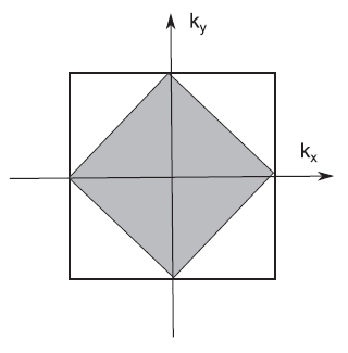
Figure 1. Fermi “surface” (line) separating the occupied from non-occupied states of the first Brillouin zone of a square lattice, at half-filling, in the tightbinding approach
Conclusion
At the other end of the spectrum. nearly free electron (NFE) model assumes that the electrons are quasi-free due to the strong hopping. Hence the only effect of the potential is felt at the boundaries of the first Brillouin zone, where the von Laue condition applies (that is, the periodic potential is only felt by electrons at the ionic coordinates). Only the terms near FBZ boundaries in Eq.(8) will be included in Eq.(11). The detailed explanation of NFE can be found in many solid state textbook. One that I like particularly is from Prof. Steven Simon’s The Oxford Solid State Basics(Chap 15). This blog ends my preparation for writing stuff about polaron theory, a topic relevant to my research. It involves QFT, statistical mechanics, and material science. Hopefully I’ll gather enough information about it for another blog soon.